A Conceptual Guide for Developers & ML Practitioners

Two stochastic parrots dressed up like Star Wars and Star Trek characters; same parrot, different costumes and roles. Image generated using Dall-E 3; prompt: Wide landscape cartoon illustration of two red-blue-yellow macaws with sunglasses on tree branches in a bright green forest. Left parrot dressed as a Jedi with robe and blue lightsaber, right parrot dressed as a classic Star Trek Vulcan officer in a gold uniform. Bold, vibrant vector style.

In my previous post I explained how LLMs are built, and how they work. In this post, I will try to explain how to adapt LLMs easily to specific tasks and domains using HuggingFace’s peft library. As explained on the official site, PEFT (Parameter-Efficient Fine-Tuning) is a family of techniques that

“only fine-tune a small number of (extra) model parameters — significantly decreasing computational and storage costs — while yielding performance comparable to a fully fine-tuned model. This makes it more accessible to train and store large language models (LLMs) on consumer hardware.”

In summary, I cover the following topics in this post:

• What task and domain adaptation of LLMs is, and which techniques are commonly used for it.
• How PEFT/LoRA works, and how it reduces the number of trainable parameters by orders of magnitude.
• Explanation of a Jupyter Notebook that implements PEFT/LoRA on a DistilBERT model for a text classification task, using the AG News dataset.

Let’s start!

Why and How Should We Adapt LLMs?

First of all, we should define some terminology:

• A Task: a specific problem we want to solve. The task is usually defined by the input and the output formats. Typically, LLMs are trained on the general task of language modeling: predicting the next word/token given an input sequence (i.e., the context); as such, they are able to generate coherent text related to the input. However, we can change their output layers (also known as heads) to perform other tasks, such as text classification (e.g., sentiment analysis and topic classification), token classification (e.g., named entity recognition or NER), etc.
• A Domain: the specific area or context to which the training texts belong and in which the task needs to be performed. Typically, LLMs are trained on a wide variety of texts from the Internet, which makes them generalists. However, we may want to adapt them to specific domains, such as medicine, finance, legal, etc. The more niche the domain, the more we may need to adapt the LLM to it to learn style, jargon, and specific knowledge.

This task and domain adaptation, although referred to as fine-tuning in the LLM world, is known as transfer learning in the context of computer vision. Howard and Ruder (2017) showed that a language model trained on a large corpus can be adapted for smaller corpora and other downstream tasks.

One common approach in the PEFT library is the Low-Rank Adaptation (or LoRA, introduced by Hu et al., 2021), which I cover in more detail in the next section. In a nutshell: LoRA freezes the pre-trained weight matrices $W$ and adds to them new matrices $dW$, which are the ones that are trained. These $dW$ matrices are factored as the multiplication of two low-rank matrices; that trick reduces trainable parameters by orders of magnitude and maintains or matches full fine-tuning performance on many benchmarks.

There are other ways to adapt LLMs which I won’t cover here, such as:

• RLHF (Reinforcement Learning with Human Feedback): This technique was used to align the initial ChatGPT model (GPT 3.5) with human preferences. Initially, human annotators ranked outputs of a GPT model. Then, these annotations were used to train a reward model (RM) to automatically predict the output score. And finally, the GPT model (policy) was trained using the Proximal Policy Optimization (PPO) algorithm, based on the conversation history (state) and the outputs it produced (actions), and using the reward model (reward) as the evaluator.
• RAG (Retrieval Augmented Generation): This method consists in outsourcing the domain-specific memory of LLMs. In an offline ingestion phase, the knowledge is chunked and indexed, often as embedding vectors. In the real-time generation phase, the user asks a question, which is encoded and used to retrieve the most similar indexed chunks; then, the LLM is prompted to answer the question by using the found similar chunks, i.e., the retrieved data is injected in the query. RAGs reduce hallucinations and have been extensively implemented recently.

In my experience, usually PEFT/LoRA and RAG are the most used techniques and they can be used in combination:

• PEFT/LoRA makes sense when we need to approach a task different than language modeling (i.e., next token prediction), or when we have a very specific domain, such as medicine or finance, which is not well represented in the general training data of the LLM.
• RAG is more useful when we have a task that can be solved by retrieving specific information, such as question answering or summarization, and when we have a large amount of domain-specific data that changes constantly. Most chatbots that are used in production for customer support, for instance, are RAG-based.

How Does PEFT/LoRA Work?

When we apply Low-Rank Adaptation (LoRA), we basically decompose a weight matrix into a multiplication of low-rank matrices that have fewer parameters.

Let’s consider a pre-trained weight matrix $W$; instead of changing it directly, we add to it a weight offset $dW$ as follows:

where

• $\hat{W}$ represents the adapted weight matrix $(d, f)$
• and $dW$ is a weight offset to be learned, of shape $(d, f)$.

However, we do not operate directly with the weight offset $dW$; instead, we factor it as the multiplication of two low-rank matrices:

where

• $A$ is of shape $(d, r)$,
• $B$ is of shape $(r, f)$,
• and $r « d, f$.

The key idea is that during training we freeze $W$ while we learn $dW$; however, instead of learning the full-sized $dW$, we learn the much smaller matrices $A$ and $B$. The forward pass of the model is modified as follows:

The proportion of weights in $dW$ as compared to $W$ is the following:

• Weights of $W$: $d \cdot f$
• Weights of $A$ and $B$: $r \cdot (d + f)$
• Proportion: $r\cdot\frac{d + f}{d \cdot f}$

Note that the number of trainable parameters is reduced by controlling the rank value $r$; for instance, if we set $r=4$, we can reduce the number of trainable parameters by more than 100x for a weight matrix of size $(4096, 4096)$.

LoRA is not applied to all weight matrices, but usually the library (peft) decides where to apply it; e.g.: projection matrices $Q$ and $V$ in attention blocks, MLP layers, etc. And, after training, we can merge $W + dW$, so there is no latency added!

In practice, LoRA assumes that the task-specific update to a large weight matrix lies in a low-dimensional subspace — and therefore can be efficiently represented with low-rank matrices.

In addition to LoRA, quantization is often applied to further reduce the model size and speed up inference. Quantization consists in reducing the precision of the weights from 32-bit floating point values to 16-bit or even 4-bit representations (as in QLoRA); in other words, high-precision floats are approximated using only k bits. This is achieved by scaling and mapping the original values to a smaller discrete set, sometimes combined with truncating less significant information. Quantization can be easily applied using the library bitsandbytes, which is very well integrated with the HuggingFace ecosystem.

Implementation Notebook

Thanks to the peft library, applying PEFT/LoRA to an LLM is very easy. The Github repository I have prepared contains the Jupyter Notebook llm_peft.ipynb, in which I provide an example.

There, I fine-tune the DistilBERT pre-trained model; DistilBERT is a smaller version of the encoder-only BERT that has been distilled to reduce its size and computational requirements, while maintaining good performance. An alternative could have been RoBERTa, which was trained roughly on 10x more data than BERT and has approximately twice the parameters of DistilBERT. We could use other models, too, e.g., generative decoder transformers like GPT-2, although in general RoBERTa seems to have better performance for classification tasks. GPT-2 is similar in size to RoBERTa.

The dataset I use is ag_news, which consists of roughly 127,600 news texts, each of them with a label related to its associated topic: 'World', 'Sports', 'Business', 'Sci/Tech' (perfectly balanced). Thus, the task head is text classification (with 4 mutually exclusive categories) and the domain is news.

The notebook is structured in clear sections and comments, which I won’t fully reproduce here; the core steps are the following:

• Dataset splitting: I divide the 127,600 samples into the sets train (108k samples), test (7.6k), and validation (12k).
• Tokenization: The AutoTokenizer is instantiated with the distilbert-base-uncased pre-trained subword tokenizer.
• Feature exploration: some exploratory data analysis is performed.
• Model setup: the AutoModelForSequenceClassification is instantiated with the distilbert-base-uncased pre-trained model, and the PeftModel is instantiated with the LoRA configuration.
• Training: the Trainer class is instantiated with the model, the TrainingArguments, and the datasets; then, the train() method is called to start training.
• Evaluation: we use the evaluate() method of the Trainer to evaluate the model on the test set, and we compute our custom metrics (accuracy, precision, recall, and F1), as defined in compute_metrics().

The feature exploration reveals that learning the classification task is going to be quite easy for the model. The function extract_hidden_states() is used to extract the last hidden states computed by the model, after each sample is passed through it. Then, these sample embeddings are mapped to 2D using UMAP, and plotted in a hexagonal plot colored by class. As we can see, each class occupies a different region in the embedding space without any fine-tuning — that is, the model already has a good understanding of the differences between the classes.

A hexagonal plot of the embeddings from the AG News dataset according to their classes. The embeddings are the last hidden states of the DistilBERT model, and they were reduced to 2D using UMAP. Image by the author.

The key aspect is the model setup for training, which is very straightforward thanks to the HuggingFace ecosystem. The code snippet below shows all the steps:

# Quantization config (4-bit for minimal memory usage)
# WARNING: This requires the `bitsandbytes` library to be installed 
# and Intel CPU and/or 'cuda', 'mps', 'hpu', 'xpu', 'npu'
bnb_config = BitsAndBytesConfig(
    load_in_4bit=True,                      # Activate 4-bit quantization
    bnb_4bit_use_double_quant=True,         # Use double quantization for better accuracy
    bnb_4bit_compute_dtype="bfloat16",      # Use bf16 if supported, else float16
    bnb_4bit_quant_type="nf4",              # Quantization type: 'nf4' is best for LLMs
)

# Transformer model: we re-instantiate it to apply LoRA
# We should get a warning about the model weights not being initialized for some layers
# This is because we have appended the classifier head and we haven't trained the model yet
model = AutoModelForSequenceClassification.from_pretrained(
    "distilbert-base-uncased",
    num_labels=len(id2label),
    id2label=id2label,
    label2id=label2id,
    quantization_config=bnb_config,
    device_map="auto"  # Optional: distributes across GPUs if available
)

# LoRA configuration
# We need to check the target modules for the specific model we are using (see below)
# - For distilbert-base-uncased, we use "q_lin" and "v_lin" for the attention layers
# - For bert-base-uncased, we would use "query" and "value"
# The A*B weights are scaled with lora_alpha/r
lora_config = LoraConfig(
    r=16,                                   # Low-rank dimensionality
    lora_alpha=32,                          # Scaling factor
    target_modules=["q_lin", "v_lin"],      # Submodules to apply LoRA to (model-specific)
    lora_dropout=0.1,                       # Dropout for LoRA layers
    bias="none",                            # Do not train bias
    task_type=TaskType.SEQ_CLS              # Task type: sequence classification
)

# Get the PEFT model with LoRA
lora_model = get_peft_model(model, lora_config)

# Define training arguments
training_args = TrainingArguments(
    learning_rate=2e-3,
    weight_decay=0.01,
    num_train_epochs=1,
    eval_strategy="steps",
    save_strategy="steps",
    eval_steps=200,
    save_steps=200,
    # This seems to be a bug for PEFT models: we need to specify 'labels', not 'label'
    # as the explicit label column name
    # If we are not using PEFT, we can ignore this argument
    label_names=["labels"],  # explicitly specify label column name
    output_dir="./checkpoints",
    per_device_train_batch_size=16,
    per_device_eval_batch_size=16,
    load_best_model_at_end=True,
    logging_dir="./logs",
    report_to="tensorboard",  # enable TensorBoard, if desired
)

# Initialize the Trainer
trainer = Trainer(
    model=lora_model,  # Transformer + Adapter (LoRA)
    args=training_args,
    train_dataset=tokenized_dataset["train"],
    eval_dataset=tokenized_dataset["validation"],
    processing_class=tokenizer,
    compute_metrics=compute_metrics,
)

After training, the model achieves an F1 score of 0.90 on the test set (compared to 0.16 before fine-tuning), which is a very good result for this task.

Other aspects are covered in the notebook, such as:

• The training can be monitored using TensorBoard.
• A predict() custom function is provided, which takes an input text, tokenizes it, passes it through the model, and decodes the predicted label.
• LoRA weights are merged and the model is persisted. Merging the LoRA weights consists in computing every $dW$ and adding them to the corresponding $W$; as mentioned before, after merging, the model can be used for inference without any latency increase.
• Some error analysis is performed by looking at the misclassified samples.
• Finally, model packaging is addressed using ONNX. This is also straightforward thanks to the HuggingFace & PyTorch ecosystem, yet essential to be able to deploy the model in production.

Summary and Conclusion

In this post, I have explained how to adapt LLMs to specific tasks and domains using Parameter-Efficient Fine-Tuning (PEFT), and more concretely, Low-Rank Adaptation (or LoRA, introduced by Hu et al., 2021). This technique allows us to train only a small number of parameters while maintaining good performance, which makes it accessible to train and store large language models on consumer hardware.

I have used the classification task applied to the AG News dataset, but many more tasks are possible: token classification (e.g., named entity recognition), question answering, summarization, etc.

Which task and domain would you like to adapt an LLM to?

I think that the HuggingFace ecosystem is incredible, as it offers plethora of pre-trained models, datasets, and libraries that make it very easy to work with LLMs, from research to production.

If you would like to deepen your understanding of the topic, consider checking these additional resources:

• LoRA: Low-Rank Adaptation of Large Language Models (Hu et al., 2021)
• Hugging Face LoRA conceptual guide
• HuggingFace Guide: mxagar/tool_guides/hugging_face
• My personal notes on the O’Reilly book Natural Language Processing with Transformers, by Lewis Tunstall, Leandro von Werra and Thomas Wolf (O’Reilly)
• My personal notes and guide for the Generative AI Nanodegree from Udacity

A Conceptual Guide for Developers & ML Practitioners

Large Language Models (LLMs) have been called stochastic parrots by some; in any case, they seem to be here to stay — and to be honest, I find them quite useful, if properly used. Image generated using Dall-E 3; prompt: Wide, landscape cartoon illustration of a happy, confident red-blue-yellow macaw wearing black sunglasses, perched on a tree branch in a green forest, with a white comic speech bubble saying "42" .

The release of ChatGPT in November 2022 revolutionized everyday life in much of the developed world. In a similar way that Google convinced us the Internet was truly useful — and that we needed their search engine — or Apple introduced the first genuinely usable smartphone that made the digital world ubiquitous, OpenAI came up with the next logical step: assistant chatbots based on Large Language Models (LLMs). Language models already existed, but OpenAI’s chat-based user interface, combined with the emergent capabilities of their huge models, led to the perfect killer app: an ever-ready genie that seems to confidently know the answer to everything.

It feels like “ask ChatGPT” has become the new “google it”.

Current LLMs are based on the Transformer architecture, introduced by Google in the seminal work Attention Is All You Need (Vaswani et al. 2017). Before that, LSTMs or Long short-term memory networks (Hochreiter & Schmidhuber, 1997) were the state-of-the-art sequence models for Natural Language Processing (NLP). In fact, many of the concepts exploited by the Transformer were developed using LSTMs as the backbone, and one could argue that LSTMs are, in some respects, more sophisticated models than the Transformer itself — if you’d like an example of an LSTM-based language modeler, you can check this TV script generator of mine.

However, the Transformer presented some major practical advantages that enabled a paradigm shift:

• Its self-attention mechanism made it possible to convert inherently sequential tasks into parallelizable ones.
• Its uncomplicated, modular architecture made it easy to scale up and adapt to many different tasks.

Simultaneously, Howard & Ruder (2018) demonstrated that transfer learning worked not only in computer vision, but also for NLP: they showed that a language model pre-trained on a large corpus could be fine-tuned for smaller corpora and other downstream tasks.

And that’s how the way to the current LLMs was paved. Nowadays, Transformer-based LLMs excel in everything NLP-related: text generation, summarization, question answering, code generation, translation, and so on.

The Original Transformer: Its Inputs, Components and Siblings

Before describing the components of the Transformer, we need to explain how text is represented for computers. In practice, text is converted into a sequence of feature vectors ${x_1, x_2, …}$, each of dimension $m$ (the embedding size or dimension). This is done in the following steps:

1. Tokenization: The text is split into discrete elements called tokens. Tokens are units with an identifiable meaning for the model and typically include words or sub-words, as well as punctuation and special symbols.
2. Vocabulary construction: A vocabulary containing all $n$ unique tokens is defined. It provides a mapping between each token string and a numerical identifier (token ID).
3. One-hot vectors: Each token is mapped to its token ID. Conceptually, this corresponds to a one-hot vector of size $n$, although in practice models operate directly on token IDs. In a one-hot vector, all cells have the value $0$ except the cell which corresponds to the token ID of the represented word, which contains the value $1$.
4. Embedding vectors: Token IDs (i.e., one-hot vectors) are mapped to dense embedding vectors using an embedding layer. This layer acts as a learnable lookup table (or equivalently, a linear projection of a one-hot vector), producing vectors of size $m$, with $m \ll n$. These embedding vectors are simply arrays of floating-point values. Typical reference values are $n \approx 100{,}000$ and $m \approx 500$.

A word/token can be represented as a one-hot vector (sparse) or as an embedding vector (dense). Embedding vectors allow to capture semantics in their directions and make possible a more efficient processing. Image by the author.

By the way, embeddings can be created for images, too, as I explain in this post on diffusion models. In general, they have some very nice properties:

• They build up a compact space, in contrast to the sparse one-hot vector space.
• They are continuous and differentiable.
• If semantics are properly captured, words with similar meanings will point in similar directions. As a consequence, we can perform arithmetic operations with them, such that algebraic operations (+, -) can be applied to words; for instance, the word queen is expected to be close to king - man + woman.

Embeddings can be computed for every modality (image, text, audio, video, etc.); we can even create multi-modal embedding spaces. If the embedding vectors capture meaning properly, similar concepts will have vectors to similar directions. As a consequence, we will be able to apply some algebraic operations on them. Image by the author.

── ◆ ──

The original Transformer was designed for language translation and it has two parts:

• The encoder, which converts the input sequence (e.g., a sentence in English) into hidden states or context.
• The decoder, which generates an output sequence (e.g., the translated sentence in Spanish) using as guidance some of the output hidden states of the encoder.

Simplified architecture of the original Transformer designed for language translation. Highlighted: inputs (sentence in English), outputs (hidden states and translated sentence in Spanish), and main parts (the encoder and the decoder).

Using as reference the figure above, here’s how the Transformer works:

• The encoder and the decoder are subdivided in N encoder/decoder blocks each; these blocks pass their hidden state outputs as inputs for the successive ones.

• The input of the first encoder block are the embedding vectors of the input text sequence. Positional encodings are added in the beginning to inject information about token order, since the self-attention layers inside the blocks (see next section) are position-agnostic. In the original paper, positional encoding vectors were $\mathbf{R} \rightarrow \mathbf{R}^n$ sinusoidal mappings: each unique scalar yielded a unique and different vector, thanks to systematically applying sinusoidal functions to the scalar. However, in practice learned positional embeddings are often used instead.

• For the translation task the encoder input contains the representation of the full original text sequence; meanwhile, the decoder produces the output sequence token by token, but it always has access to the full and final encoder hidden states (the context).

• The decoder blocks work in a similar way as the encoder blocks; the last decoder block produces the final set of hidden states, which are mapped to output token probabilities using a linear layer followed by a softmax function (i.e., we have a classification head over the vocabulary).

Soon after the publication of the original encoder-decoder Transformer designed for the language translation task, two related, important Transformers were introduced:

• BERT: Pre-training of Deep Bidirectional Transformers for Language Understanding (Devlin et al., 2018), which is an implementation of the encoder-only part of the original Transformer.
• GPT: Improving Language Understanding by Generative Pre-Training (Radford et al., 2018), an implementation of the decode-only part of the original Transformer.

BERT-like encoder-only transformers are commonly used to generate feature vectors $x$ of texts which can be used in downstream applications such as text or token/word classification. If the Encoder is trained separately, the sequence text is shown to the architecture with a masked token which needs to be predicted. This scheme is called masked language modeling.

GPT-like decoder-only transformers are commonly used as generative models to predict the next token in a sequence, given all the previous tokens (i.e., the context, which includes the prompt). During training, the model is shown sequences of text and learns to predict each token based on the preceding ones.

The full encoder-decoder architecture is not as common as the other two currently, but it is used in some specific models for text-to-text tasks, such as summarization and translation. Examples include T5 (Raffel et al., 2019) and BART (Lewis et al., 2019).

Deep Dive into the Transformer Architecture

So far, we’ve seen the big picture of the Transformer architecture and its subtypes (encoder-decoder, encoder-only, decoder-only).

But what’s inside those encoder and decoder blocks? Just Attention, normalization, and linear mappings. Let’s see them in detail.

The Transformer architecture with all its components. Image from the orinal paper by Vaswani et al. (2017), modified by the author.

As we can see in the figure above, each of the N encoder and decoder blocks are composed of the following sub-components:

• Multi-Head Self-Attention modules: The core component of the Transformer. It allows the model to focus on different parts of the input sequence when processing each token. Multiple attention heads enable the model to capture various relationships and dependencies in the data. More on this below :wink:
• Skip connections, Add & Norm: These are residual (skip) connections followed by layer normalization. Residual connections help to avoid vanishing gradients in deep networks by allowing gradients to flow directly through the skip connections. Normalizing the inputs across the features dimension stabilizes and accelerates training.
• Feed-Forward Neural Network (FFNN, i.e., several concatenated linear mappings): A fully connected feed-forward network applied independently to each position. It consists of two linear transformations with a ReLU activation in between, allowing the model to learn complex representations.

The key contribution of the Transformer architecture is the Self-Attention mechanism. Attention was introduced by Bahdanau et al. (2014) and it allows the model to weigh the importance of different tokens in the input sequence when processing each token. In practice for the Transformer, similarities of the tokens in the sequence are computed simultaneously (i.e., dot product) and used to weight and sum the embeddings in successive steps.

We can see there are different types of attention modules in the Transformer:

• Self-Attention in the encoder blocks: Each token attends to the similarities of all tokens in the input sequence. It’s called self-attention, because the similarities of the input tokens only are used, i.e., without any interaction with the decoder. For more information, keep reading below.
• Masked Self-Attention in the decoder blocks: Each token attends to all previous tokens in the output sequence (masked to prevent attending to future tokens).
• Encoder-Decoder Cross-Attention in the decoder blocks: Each token in the output sequence attends to all tokens in the encoder-input sequence. In other words, all final hidden states from the encoder are used in the attention computation.

Additionally, each attention module is implemented as a Multi-Head Attention mechanism. This means that multiple attention heads are used in parallel. The following figure shows brief overview of how this works.

The LLM (Self-)Attention module, annotated. Image by the author.

The Self-Attention Head is the core implementation of the attention mechanism in the Transformer. Each multi-head attention module contains $n$ self-attention heads, which operate in parallel. The input embedding sequence $Z$ is passed to each of these $n$ self-attention heads, where the following occurs:

• We transform the original embeddings $Z$ into $Q$ (query), $K$ (key), and $V$ (value). The transformation is performed by linear/dense layers ($W_Q$, $W_K$, $W_V$), which consist of the learned weights. These query, key, and value variables come from classical information retrieval; as described in NLP with Transformers (Tunstall et al., 2022), using the analogy to a recipe they can be interpreted as follows:
  • $Q$, queries: ingredients in the recipe.
  • $K$, keys: the shelf-labels in the supermarket.
  • $V$, values: the items in the shelf.
• $Q$ and $K$ are used to compute similarity scores between token embeddings (self dot-product), and then we use those similarity scores to weight the values $V$, so the relevant information is amplified. This can be expressed mathematically with the popular and simple attention formula: \(Y = \mathrm{softmax}(\frac{QK^T}{\sqrt{d_k}})V,\) where
  • $Y$ are the contextualized embeddings,
  • and $d_k$ is the dimension of the key vectors (used for scaling), which is the same as the embedding size divided by the number of heads (head dimension).

Then, these $Y_1, …, Y_n$ contextualized embeddings are concatenated and linearly transformed to yield the final output of the multi-head attention module. The output of the first multi-head self-attention module is the input of the next one, and so on, until all $N$ blocks process embedding sequences. Note that the output embeddings from each encoder block have the same size as the input embeddings, so the encoder block stack has the function of transforming those embeddings with the attention mechanism.

I hope it is now clear why the Transformer paper is titled Attention Is All You Need: It turns out that successively focusing and transforming the embeddings via the attention mechanism produces the magic in the LLMs.

Finally, let’s see some typical size values, for reference:

• Embedding size: 768, 1024, …, 2048.
• Sequence length (context, number of tokens): 128, 256, …, 8192.
• Number of layers/blocks, $N$: 12, 24, 36, 48.
• Number of attention heads, $n$: 12, 16, 20, 32.
• Head dimension: typically, embedding size divided by number of heads.
• Feed-Forward Network (FFN) inner dimension: 2048, 4096, …, 10240.
• Vocabulary size, $m$: 30,000; 50,000; 100,000; 200,000.
• Total number of parameters: from 110 million (e.g., BERT-base) to 175 billion (e.g., GPT-3), and much more!

Using the Transformer Outputs

There are many ways in which the outputs of the Transformer can be used, depending on the task and the architecture (some of these ways were mentioned above already):

• Encoder-decoder models (e.g., T5 (Raffel et al., 2019)) have been used for text-to-text tasks, such as translation and summarization. However, big enough decoder-only models (e.g., GPT-3 (Brown et al., 2020)) have shown remarkable performance in these tasks, too, and have become more popular nowadays.
• Encoder-only models (e.g., BERT (Devlin et al., 2018)) are commonly used to generate feature vectors of texts, which can be used in downstream applications such as text or token/word classification, or even regression. We just need to attach the proper mapping head to the output of the encoder (e.g., a linear layer for classification) and fine-tune the model on the specific task.
• Decoder-only models (e.g., GPT-3 (Brown et al., 2020)) are commonly used as generative models to predict the next token in a sequence, given all the previous tokens (i.e., the context, which includes the prompt).

Probably, the most common way to interact with LLMs for the layman user is the latter: decoder-only generative models. As mentioned, these models generate one word/token at a time, so we feed their outputs back as inputs for successive generations (hence, they are called autoregressive). In that scheme, we need to consider the following questions:

1. Which tokens are considered as candidates every generation? (token sampling)
2. What strategy is used to select and chain the tokens? (token search during decoding)

Recall that the output of the generative model is an array of probabilities, specifically, a float value $p \in [0,1]$ for each item in the vocabulary set $V$. A naive approach would be to

1. consider all token probabilities as candidates ${p_1, p_2, …}$ (full distribution sampling),
2. and select the token with the highest probability at each generation step: $\mathrm{token} = V(\mathrm{argmax}{p_1, p_2, …})$ (greedy search decoding).

However, such a naive approach often leads to repetitive and dull text generation, as described by Holtzman et al. (2019). To mitigate this issue, these parameters and strategies are often used:

• Temperature: we apply the softmax function to the output logits $z_i = \mathrm{ln}(p_i)$ by using a temperature variable $T$ in the exponent (Boltzman distribution): $p_i’ = \mathrm{softmax}(z_i / T)$. That changes the $p$ values as follows:
  • $T = 1$: no change, same as in the original output.
  • $T < 1$: small $p$-s become smaller, larger $p$-s become larger; that means we get a more peaked distribution, i.e., less creativity and more coherence, because the most likely words are going to be chosen.
  • $T > 1$: small $p$-s become bigger, larger $p$-s become smaller; that yields a more homogeneous distribution, which leads to more creativity and diversity, because any word/token could be chosen.
• Top-$k$ and top-$p$: instead of considering all tokens each with their $p$ (with or without $T$), we reduce it to the $k$ most likely ones and select from them using the distribution we have; similarly, with a top-$p$, we can select the first tokens that cumulate up to a certain $p$-threshold and choose from them.
• Beam search decoding (as oposed to greedy search): we select a number of beams $b$ and keep track of the most probable next tokens building a tree of options. The most likely paths/beams are chosen, ranking the beams with their summed log probabilities. The higher the number of beams, the better the quality, but the computational effort explodes. Beam search sometimes suffers from repetitive generation; one way to avoid that is using n-gram penalty, i.e., we penalize the repetition of n-grams. This is commonly used in summarization and machine translation.

Token sampling strategies in LLMs. The LLM outputs a probability for each of the tokens in the vocabulary. If we apply a temperature T, top-k, or top-p strategy, we modify the distribution from which the next token is sampled. With T > 1, the distribution becomes more uniform, leading to more diverse outputs (since tokens have a more similar probability); in contrast, with T < 1, the distribution becomes more peaked, leading to more focused and coherent outputs. If we set top-k to be 3, we only consider the three most likely tokens for sampling; similarly, with a top-p threshold of 80%, we consider the smallest set of tokens whose cumulative probability is at least 80%. Image by the author.

Additional Relevant Concepts

My goal with this post was to explain in plain but still technical words how LLMs work internally. In that sense, I guess I have already given the best I could and I should finish the text. However, there are some additional details that probably fit nicely as appendices here. Thus, I have decided to include them with a brief description and some references, for the readers who optionally want to go deeper into the topic.

── ◆ ──

Context Size — This refers to the maximum number of words/tokens that the model can consider as input at once, i.e., the input sequence length or seq_len. If we look at the attention mechanism figure above, we will see that the learned weight matrices are independent of the context size; however, the attention computation itself scales quadratically with sequence length due to the $QK^T$ operation. This is a major bottleneck in terms of memory and speed, and it’s the main reason why the initial LLMs had a fixed and shorter context size ($512$ - $4,096$ tokens). In recent years, the research community has explored new methods to alleviate that limitation, introducing techniques such as sparse attention, linearized attention, low-rank approximations, and other mathematical/architectural/system tricks. These enable larger context sizes (up to $1,000,000$ tokens in the case of Gemini Pro).

Distillation and Quantization — As their name indicates, Large Language Models are large, and that makes them difficult to deploy in production environments. Two techniques to overcome that are distillation and quantization. When we distill a model, we train a smaller student model to mimic the behavior of a larger, slower but better performing teacher (i.e., the original LLM). This is achieved, among other techniques, by using the teacher’s output probabilities as soft labels when training the student. A notable example of distillation is DistilBERT (Sanh et al., 2019), which achieves around 97% of BERT’s performance, but with 40% less memory and 60% faster inference. On the other hand, quantization consists in representing the weights with lower precision, i.e., float32 -> int8 ($32/8 = 4$ times smaller models). The models not only become smaller, but the operations can be done faster (even 100x faster), and the accuracy is sometimes similar.

Emergent Abilities — As described by Wei et al. (2022), “emergent abilities are those that are not present in smaller models, but appear in larger ones”. In other words, they are capabilities that arise, but which were not explicitly trained. This often referred to as zero-shot or few-shot learning, because the model can perform tasks without any or with very few examples, as demonstrated by GPT-3 (Brown et al., 2020), and they start to appear in the 10-100 billion parameter range (GPT-3 had 175 billion parameters). Examples of emergent abilities include arithmetic, commonsense reasoning, and even some forms of creativity.

Scaling Laws — Kaplan et al. published in 2020 the interesting paper Scaling Laws for Neural Language Models, which describes how the performance of language models scales. They discovered that there is a power-law relationship between the model’s performance measured in terms of loss $L$, the required compute $C$, the dataset size $D$ and the model size $N$ (number of parameters): $L(X) \sim X^{-\alpha}$, with $X \in {N, C, D}$ and $\alpha \in [0.05, 0.1]$. In other words, when model size $N$, dataset size $D$, or training compute $C$ are scaled independently (and are not bottlenecks), the training loss $L$ decreases approximately as a power law of each quantity. In that sense, we can use these scaling laws to extrapolate model performance without building them, but theoretically! Similarly, for a fixed compute budget, there is an optimal trade-off between model size and dataset size. These insights led to the development of more efficient training strategies and architectures, such as the ones explored in the Chinchilla study (Hoffman et al., 2022), which suggest that smaller models trained on more data can achieve better performance than larger models trained on less data. Finally, note that training compute is roughly proportional to $6 \times N \times D$, while inference compute scales linearly with model size and generated sequence length.

RLHF: Reinforcement Learning with Human Feedback — OpenAI presented InstructGPT (Ouyang et al., 2022) shortly before releasing their popular ChatGPT. This paper explains how the initial chatbot model GPT 3.5 was aligned with human preferences using reinforcement learning. They followed 3 major steps: (1) First, a GPT model was fine-tuned with human-written conversation input-output pairs. (2) Then, the GPT model produced several answers to a set of prompts and human annotators ranked these outputs from best to worst. These annotations were used to train a reward model (RM) to automatically predict the output score. (3) Finally, the GPT model (policy) was trained using the Proximal Policy Optimization (PPO) algorithm, based on the conversation history (state) and the outputs it produced (actions), and using the reward model (reward) as the evaluator.

PEFT: Parameter-Efficient Fine-Tuning — Low-Rank Adaptation of Large Language Models (or LoRA by Hu et al., 2021) consists in applying a mathematical trick during the fine-tuning of LLMs to make the process much more efficient. The pre-trained weight matrices $W$ are frozen and we add to them the new matrices $dW = A \cdot B$, which are the ones trained. These are factored as $dW = A \cdot B$, having $A$ and $B$ a much lower rank. The trick reduces trainable parameters by orders of magnitude and maintains or matches full fine-tuning performance on many benchmarks. Therefore, it has become a standard method for domain adaptation and instruction tuning. One popular implementation is the peft library from HuggingFace.

RAG: Retrieval Augmented Generation — LLMs have humongous amounts of general knowledge encoded in their parameters, but need to be fine-tuned for specific domains. That process is cumbersome and often inefficient, particularly when domain-specific information changes frequently. The work Retrieval-Augmented Generation (RAG) for Knowledge-Intensive NLP Tasks (Lewis et al., 2020) addressed such settings by using non-parametric information, i.e., they outsource the domain-specific memory. It works as follows: in an offline ingestion phase, the knowledge is chunked and indexed, often as embedding vectors. In the real-time generation phase, the user asks a question, which is encoded and used to retrieve the most similar indexed chunks; then, the LLM is prompted to answer the question by using the found similar chunks, i.e., the retrieved data is injected in the query. RAGs reduce hallucinations and have been extensively implemented recently.

Reasoning Models — Wei et al. showed that Chain-of-Thought Prompting Elicits Reasoning in Large Language Models (2022). In other words, prompting the model to think step by step improves its performance on math and reasoning tasks, suggesting that reasoning abilities are partly latent in large models. That simple yet powerful idea sparked research into prompting strategies and powered the fine-tuning with objectives that encourage multi-step inference, structured thinking, and tool use. One of the first popular open source reasoning models was DeepSeek-R1, but most of the current models have all improved reasoning capabilities, either by scale or via fine-tuning with reasoning objectives.

Agents — The improvement of reasoning capabilities and tool usage boosted the development of the so-called agentic workflows. An agent is basically an LLM which has tool access and is allowed to perform actions, e.g., read our emails and do some processing with them, like classify or even answer the trivial ones. Libraries like LangChain and LangGraph have made it relatively easy to build multi-agent systems that perform increasingly complex workflows, and frameworks like OpenClaw have enabled the creation of personalized assistants. The future is being automated, and agents seem to be a key part of that — security issues aside.

Summary and Some Final Thoughts

Large Language Models are not magic. At their core, they are stacks of linear transformations, normalization layers, and attention mechanisms applied to sequences of embedding vectors. And yet, by scaling those simple components to unprecedented sizes (in terms of parameters, data, and compute) they exhibit capabilities that feel surprisingly powerful.

In this post, I have:

• Reviewed how text is converted into embedding vectors.
• Described the original encoder-decoder Transformer and its encoder-only and decoder-only variants.
• Taken a closer look at the self-attention mechanism and multi-head attention.
• Discussed how decoding strategies such as temperature, top-$k$, top-$p$, and beam search influence text generation.
• Briefly touched on important side concepts such as context length, scaling laws, RLHF, PEFT/LoRA, RAG, reasoning models, and agents.

If you want to go deeper into the topic, I recommend the following resources:

• The original paper: Attention Is All You Need (Vaswani et al., 2017)
• My notes of the great book NLP with Transformers (Tunstall et al., 2022)
• The Illustrated Transformer (Jay Alammar)
• The Annotated Transformer (Harvard NLP)
• A minimal PyTorch re-implementation of the OpenAI GPT (Andrej Karpathy)

── ◆ ──

LLMs have increased my productivity significantly. I use them extensively for research, text editing, and programming. However, I still think that they are expert systems for experts: when used without proper guidance, the quality of their output can be quite mediocre — and in some cases, even worse: I have seen many instances of dull AI-generated texts and bloated, unmaintainable code. I am aware, of course, that they are improving at a rapid pace, though.

Overall, I am optimistic. In the same way that the Internet increased our overall productivity — while replacing some jobs and creating new ones — I think LLMs will probably have a similar (or even greater) net-positive effect. For instance, I do not believe that Software Engineers will disappear. Rather, they will likely shift toward tasks related to architecture, orchestration, integration, and maintenance. Junior roles and inexperienced professionals seem to be the most affected at the moment, but they will also be able to learn faster with these tools than we did before. As the ecosystem stabilizes, they may end up being in even higher demand. And, at the end of the day, everyone will want a human responsible for any AI-generated outcome.

I am confident that we will find ways to mitigate risks such as dependence, personal data harvesting and automated control/surveillance, just as we invented gyms to stay fit and healthy, or engineered locks and cryptographic systems to protect our privacy. At the moment, it is hard for me to believe that a Transformer-based model can intentionally go rogue and cause harm on its own, because I cannot conceive of any consciousness in them — at least not in the sense of “I am aware that I exist here and now, and I have some purpose and agency”. I see LLMs as systems that simulate patterns from their training data. In contrast, humans maintain (and constantly update) a world model, and use language as a tool to interact with that world model. An LLM has no internal state and it can’t learn in real-time — it can only simulate “small breaths” by producing tokens; one could even argue that it even “dies” after producing each token, or at least once the final <STOP> token is emitted.

At the same time, granting an LLM-based agent unrestricted access to personal information and powerful tools could indeed be irresponsible — perhaps comparable to giving a monkey a machine gun. Yet we have faced similar situations in the past: when technologies become powerful, we introduce safeguards, norms, and regulation to govern their use.

Let’s see what the future awaits us. I believe it will be exciting, and that we will find ways to navigate the limitations and risks of this technology, as we’ve done in the past.

How have LLMs impacted your life? How do you think they will change the world in the next 5-10 years?

Hands-On Examples with HuggingFace

An AI drawing an AI drawing an AI... Image generated using Dall-E 3. Prompt: A friendly humanoid robot sits at a wooden table in a bright, sunlit room, happily drawing on a sketchbook. Soft light colors, landscape, peaceful, productive, and joyful atmosphere. The robot is drawing an image of itself drawing, creating a recursive effect. Large window in the background with greenery outside, warm natural lighting.

In just a few years, image generation has gone from “cool demo” to an almost ubiquitous tool. Variational Autoencoders (VAEs - Kingma & Welling, 2013) were followed by Generative Adversarial Networks (GANs - Goodfellow et al., 2014), and finally Denoising Diffusion Probabilistic Models (DDPMs - Ho et al., 2020) became the dominant approach, leading to systems like Stable Diffusion XL (Podell et al., 2023) or Imagen & Nano Banana.

In the first post of this series, I explain how these model families work and I walk through a minimal DDPM implementation. That DDPM is trained on car images and produces outputs like these:

Output of a Denoising Diffusion Probabilistic Model (Ho et al., 2020) consisting of 54 million parameters, trained on the Stanford Cars Dataset (16,185 color images resized to 64x64 pixels) for 300 epochs. Check the complete implementation here.

In this second part, I’ll focus on the practical use of diffusion models, specifically, on using the invaluable tools provided by HuggingFace. To that end, I’ve divided the post in three parts:

1. A brief introduction to HuggingFace.
2. A hands-on dive into some examples with HuggingFace Diffusers.
3. A small in-painting application that puts everything together.

Let’s go!

A Very Brief Introduction to HuggingFace

HuggingFace has become one of the most important hubs in the machine learning community. It provides a collaborative environment where state-of-the-art datasets and models can be shared, explored and even tried directly from the browser (via Spaces). Beyond models and datasets, HuggingFace offers two particularly powerful resources:

• courses, covering key domains and techniques such as computer vision, natural language processing, audio, agents, 3D processing, reinforcement learning, and more;
• and a rich ecosystem of libraries that let us work with datasets and models end-to-end, across modalities. The most relevant ones for this post are:
  • datasets: access, share, and process audio, text, and image datasets.
  • transformers: training and inference for text, vision, audio, video, and multimodal models.
  • diffusers: pre-trained diffusion models for generating images, videos, and audio.

All of these can be installed easily in a Python environment:

pip install datasets transformers diffusers["torch"] accelerate gradio

Screenshot of the HuggingFace portal, showing available models sorted by their popularity.

In practice, discriminative models (across all modalities) and generative models for text are usually handled via the transformers library. On the other hand, generative diffusion models are managed through diffusers.

Models can be browsed and selected directly from the HuggingFace website, where they can be filtered by several criteria. One of the most useful is the task, for example:

• sentiment-analysis
• text-generation
• summarization
• translation
• audio-classification
• image-to-text
• object-detection
• image-segmentation
• …

If we click on a model we will land on its model card page, which typically includes evaluation metrics, references, licensing information, and often a short code snippet showing how to load and run the model.

Pipelines

The easiest way to run inference with most HuggingFace models is through the pipeline interface. While each task has its own specifics, the overall pattern is remarkably consistent. As an example, here’s how a text-generation pipeline looks:

import transformers

# Load the pipeline
pipe = transformers.pipeline(
    "text-generation",  # task
    model="Organization/ConcreteModel",  # change to real model, e.g.: "openai-community/gpt2"
)

# Define the input (prompt)
messages = [
    {"role": "system", "content": "You are an AI who can draw AIs."},
    {"role": "user", "content": "What's the best technique to draw an AI?"},
]

# Generate output (text)
outputs = pipe(
    messages,
)

# Display output (text)
print(outputs[0]["generated_text"][-1])

From this (deliberately simplified) example, we can extract a common workflow:

• First, a model pipeline is loaded, by defining the task family (e.g., text-generation) as well as the concrete model name (e.g., openai-community/gpt2) we want to use.
• Then, we need to define the input to the pipeline; the input depends on the task at hand: if we want to classify an image, we need to load an image; if we want to generate text, we need an initial prompt of conversation history, etc.
• Finally, we pass the input to the pipeline and collect the output. The output format again depends on the task.

Instead of relying on the generic pipeline abstraction, we can also load a specific model class directly. This is particularly common when working with diffusion models. For example, a typical text-to-image setup using diffusers looks like this:

from diffusers import ConcreteModel   # change to real model, e.g.: AutoPipelineForText2Image

# Load the pipeline
pipe = ConcreteModel.from_pretrained(
    "Organization/ConcreteModel",  # change to real model, e.g.: "stabilityai/sdxl-turbo"
    ...
)

# Define the input (prompt)
prompt = "An AI drawing an AI"

# Generate output (image)
image = pipe(
    prompt=prompt,
    ...
).images[0]

# Save output (image)
image.save("example.png")

More Information on the HuggingFace Ecosystem

This brief overview barely scratches the surface of the HuggingFace ecosystem. In the next sections, I’ll focus on concrete, ready-to-use examples that build directly on these ideas.

If you’d like to explore further, here are some additional resources:

• My guide on HuggingFace, which covers topics such as:
  • Combining models with Pytorch/Tensorflow code.
  • More complex pre- and post-processing steps for each task/modality, e.g.: tokenization, encoding, etc.
  • Fine-tuning pre-trained models for different tasks by adding custom heads.
  • Saving/loading fine-tuned models locally, as well as exporting them as ONNX for production.
  • Examples with generative models of all modalities and conditioning types: text-generation, text-to-image, text-to-video, etc.
• A comprehensive example in which I fine-tune a Large Language Model (LLM) to perform a custom text classification task.
• My notes on the exceptional book Natural Language Processing (NLP) with Transformers (Tunstall, von Werra & Wolf — O’Reilly), written by the co-founders of HuggingFace — highly recommended if you want to use transformers effectively.

HuggingFace Diffusers in Practice

Let’s now move from concepts to code and run a few concrete examples using the diffusers library. For this section, I’ve prepared a companion notebook:

:point_right: diffusers/diffusers_and_co.ipynb

In this post, I’ll focus on showing and discussing the results produced by different models. If you want to see the full (and commented) code, I recommend opening the notebook alongside the article.

:warning: Hardware note: To run the notebook locally, you’ll need a GPU setup with at least 12 GB of VRAM. As an alternative, you can use a Google Colab instance with a NVIDIA T4, or similar.

Stable Diffusion XL Turbo

The first example in the notebook covers a conditioned image generation task, specifically text-to-image, using the Stable Diffusion XL Turbo model. The code closely follows the patterns introduced in the previous section:

from diffusers import AutoPipelineForText2Image

# Load the SDXL-Turbo text-to-image pipeline
pipe = AutoPipelineForText2Image.from_pretrained(
    "stabilityai/sdxl-turbo", 
    torch_dtype=torch.float16, 
    variant="fp16"
)

prompt = """
A friendly humanoid robot sits at a wooden table in a bright, sunlit room, happily drawing on a sketchbook.
Soft light colors, landscape, peaceful, productive, and joyful atmosphere.
The robot is drawing an image of itself drawing, creating a recursive effect.
Large window in the background with greenery outside, warm natural lighting.
"""

# Seed for reproducibility
rand_gen = torch.manual_seed(148607185)

# Generate an image based on the text prompt
image = pipe(
    prompt=prompt, 
    num_inference_steps=1, # 1 for sdxl-turbo, 25-50 for SD
    guidance_scale=1.0, # 1 for sdxl-turbo, 6-10 for SD
    negative_prompt=["overexposed", "underexposed"], 
    generator=rand_gen
).images[0]

The result is already quite impressive, but it also clearly reveals its synthetic nature. Subtle artifacts appear in areas like eyes and fingers, and some mechanical structures lack global consistency or realism — typical issues when pushing generation speed to the extreme.

Image generated with SDXL Turbo. Prompt: A friendly humanoid robot sits at a wooden table in a bright, sunlit room, happily drawing on a sketchbook. Soft light colors, landscape, peaceful, productive, and joyful atmosphere. The robot is drawing an image of itself drawing, creating a recursive effect. Large window in the background with greenery outside, warm natural lighting.

Stable Diffusion XL Turbo is a real-time text-to-image diffusion model derived from Stable Diffusion XL (SDXL). Its key feature is that it can generate images in as few as one to four denoising steps. Unlike traditional diffusion models (which often require dozens of inference steps) SDXL Turbo prioritizes latency and interactivity, while still preserving much of SDXL’s visual quality.

This speedup is achieved through Adversarial Diffusion Distillation (ADD):

• A large, high-quality SDXL model acts as a teacher.
• The Turbo model is trained to match the teacher’s output distribution.
• An adversarial objective helps close the quality gap introduced by aggressive step reduction.

In short, a large model is distilled into a much faster one, enabling real-time image generation in creative tools and user interfaces.

Playground V2

An interesting alternative to SDXL Turbo is Playground V2. This model also targets high-quality image generation with fewer inference steps, but it takes a different approach: it prioritizes visual quality and aesthetics and it does not rely on distillation during training. Using the same prompt, Playground V2 produces a different output:

Model: Playground V2. Same prompt ad before: A friendly humanoid robot sits at a wooden table...

Combining Models

Diffusion models don’t have to be used in isolation — they can also be chained together! In the next example, SDXL Turbo first generates an image of a puppy. That image is then used as conditioning input for the image-to-image model Kandinsky 2.2. The result is an exaggerated image of a dog, but I think it showcases the potential of building such compositional pipelines.

Left image generated by SDXL Turbo. Right image generated by Kandinsky Prior 2.2. Left prompt: A painting of a friendly dog painted by a child. Right prompt: A photo of a friendly dog. High details, realistic (negative: low quality, bad quality).

Kandinsky is a multimodal diffusion model that separates semantic understanding from image generation. Unlike SDXL-style models, which directly condition image generation on text embeddings, Kandinsky uses a two-stage architecture:

• Prior model, which maps text (and optionally images) into a shared latent space that represents high-level semantics.
• Decoder model (diffusion), which takes these semantic embeddings and generates the final image via a diffusion process.

This explicit separation makes Kandinsky particularly well suited for compositional pipelines. One such pipeline consists in in-painting, i.e.: we ask the model to generate a sub-image on a provided initial image. Here’s how it works:

• Mask definition: A binary mask specifies which regions of the image should be regenerated (white) and which should remain fixed (black).
• Latent conditioning: The unmasked parts of the image are encoded and injected into the diffusion process, anchoring the generation spatially.
• Semantic guidance via the prior: Text prompts and optional image context guide what should appear in the masked regions.
• Diffusion-based regeneration: Noise is added only in the masked area, and the model denoises it while respecting both the surrounding visual context and the semantic intent from the prompt.

Because Kandinsky reasons at a semantic level first, inpainting results tend to be context-aware: lighting, perspective, and style are usually consistent with the original image, even when the prompt introduces new elements.

Here’s an example with the popular oil painting The Girl with the Pearl Ear-ring from Vermeer. Unfortunately, the pearl ear-ring doesn’t survive the process :sweat_smile:

Model: Kandinsky Inpaint 2.2. Prompt: Oil painting of a woman wearing a surgical mask, Vermeer (negative: bad anatomy, deformed, ugly, disfigured). I obtained the image from the Wikipedia and draw the mask manually. Check this piece from Banksy, if you would like to know how this could be done differently.

Building Proof-of-Concept Applications: Zero-Shot Segmentation and In-Painting

As shown in the notebook diffusers/diffusers_and_co.ipynb, running different models for isolated tasks is already quite straightforward. This naturally leads to the next question:

What if we combine several models to build small, interactive applications?

Along these lines, I implemented a simple proof-of-concept: inpainting_app. The idea behind it is to chain segmentation and diffusion-based in-painting into a single workflow:

• First, we load an image and select a few points on the region we want to modify (typically the foreground).
• Next, the Segment Anything Model (SAM) from Meta generates a segmentation mask for that region. Everything outside the mask is treated as background. SAM is a vision transformer capable of zero-shot segmentation, but it still requires some minimal guidance (points or a bounding box) to specify the region of interest.
• Finally, we select either the foreground or the background region and run the in-painting version of SDXL model. The selected region is regenerated according to a text prompt, while remaining visually consistent with the rest of the image.

As before, if you plan to run the app locally you’ll need a GPU setup with at least 12 GB of VRAM :sweat_smile:.

UI and Application Structure

The application is built using Gradio, a Python library similar to Streamlit which builds nice-looking, web-based GUIs. Since Gradio is developed by HuggingFace, it integrates seamlessly with the models used here.

If you want a deeper introduction to Gradio, you can check my Gradio Quickstart Guide, where I cover the basics and several advanced patterns.

The structure of the app is intentionally simple:

• The GUI and the app structure are controlled by app.py. The entry point is app.generate_app(), which takes two functions as inputs:
  • a function that performs image segmentation given a set of user-selected points,
  • and a function that runs in-painting given an image, a mask, and a prompt.
• The notebook inpainting.ipynb defines and prepares those input functions:
  • run_segmentation(raw_image, input_points, processor, model, ...) -> input_mask
  • run_inpainting(raw_image, input_mask, prompt, pipeline, ...) -> generated_image
• Internally, app.generate_app() creates a gradio.Blocks layout, which is composed of gradio.Row() sections that contain the UI widgets: image canvases, sliders, text boxes, buttons, etc. These widgets are connected to callback functions; for instance: when we select points in the uploaded raw_image, the callback on_select() is invoked, which under the hood executes run_segmentation() using the uploaded raw_image and the selected input_points.

While everything could be packaged into standalone modules, keeping part of the logic in a notebook makes experimentation much easier and encourages rapid iteration.

The Result

When the application is launched via app.generate_app(), the user sees the following UI in http://localhost:8080:

The Graphical User Interface (GUI) or our application.

So how does it perform? Let’s look at an example.

Monalisa re-imagined. SAM (Segment Anything Model) is used to segment foreground (green) & background (yellow), and Stable Diffusion XL Inpainting to re-generate the selected region. Prompt (applied to the background): A fantasy landscape with flying dragons (negative: artifacts, low quality, distortion).

I think that the result shows that the pipeline produces a visually coherent image: the new background blends naturally with the original painting’s lighting, perspective, and color palette. Despite the strong semantic change introduced by the prompt, the Mona Lisa remains intact and consistent, which highlights how well segmentation and diffusion-based in-painting can work together even in artistic, non-photographic domains.

Wrap Up

In this second post, we moved from theory to practice and explored how modern diffusion models can be used out of the box with HuggingFace tools. I covered how to run state-of-the-art text-to-image models with diffusers, how different diffusion architectures trade off speed and quality, and how combining models enables more powerful workflows such as segmentation-aware in-painting.

Beyond individual examples, the main takeaway is how composable today’s generative models have become. By chaining pre-trained components—segmentation, conditioning, and diffusion—we can quickly prototype creative and practical applications without training models from scratch.

If you want to dig deeper, here are some useful starting points:

• :point_right: Conceptual background on diffusion models (Part 1 of this series)

• :point_right: Code for this post (Diffusers examples)

• :point_right: In-painting application (SAM + SDXL)

• :point_right: My guide on HuggingFace

I’m curious to hear your thoughts:

What real-world or creative use case do you think would benefit most from this kind of segmentation-guided in-painting app? Do you know some businesses using similar pipelines?

A Conceptual Guide for Developers & ML Practitioners

Fascinating Milky Way over Dolomite mountains. Was all this spontaneous generation? Which is its latent space? Photo by @felixrottmann from Unsplash.

I still find it fascinating that machine learning models are able to learn from examples, even after working with them for more than a decade.
But what truly feels like magic to me are image and video generation models.

Driven by that fascination, I decided to write a short series of posts explaining how these models work, both in theory and in practice.

In this first post, you will:

• Learn how image generation differs from image discrimination (e.g., image classification).
• Understand how Diffusion models compare to Generative Adversarial Networks (GANs) and Variational Autoencoders (VAEs).
• Learn how Denoising Diffusion Probabilistic Models (DDPMs) work at both conceptual and mathematical levels.
• See a full, minimal PyTorch implementation of a DDPM that generates car images using a consumer-grade GPU.

In the second and final post, I’ll move on to practical examples using the Hugging Face libraries.

Let’s get started!

── ◆ ──

In machine learning, any sample or data instance can be represented as feature vector $x$. These features could be the RGB values of an image’s pixels or the words (tokens) of a text represented as vocabulary indices. In deep learning, these vectors are often transformed into embeddings or latent vectors, which are compressed representations that still retain differentiable semantic meaning.

Any sample or data point of any modality can be represented as an n-dimensional vector x in machine learning; in the figure, images and words (tokens) are represented as 2D vector embeddings. These embeddings contain conceptual information in a compressed form. When semantics and/or similarities between samples are captured, algebraic operations can be used with the vectors, resulting in coherent, logical outputs. Image by the author.

Up until recently, mainly discriminative models have been used, which predict properties of those embeddings. These models are trained with annotated data, for instance class labels: $x$ belongs to class $y = $ cat or dog. The model then learns decision boundaries that allow it to predict the class of new, unseen samples. Mathematically, we can represent that as $y = f(x)$, or better as $p(y \mid x)$, i.e., the probability $p$ of each class $y$ given the instance/sample $x$.

On the other hand, in the past years, generative models have gained popularity. These models do not explicitly capture decision boundaries; instead, they learn the probability distribution of the data. As a result, they can sample from these distributions and generate new, unseen examples. Following the same mathematical notation, we can say that the models learn $p(x)$ or $p(x, y)$, if the classes are considered.

A dataset of 2D samples $x$ (i.e., 2 features) used to fit a discriminative and a generative model. Discriminative models learn decision boundaries and are able to predict the class $y$ of new, unseen instance. Generative models learn the data distribution $p(x)$ and are able to sample new unseen instances. Image by the author.

In terms of ease of control, generative models can be of two main types:

• Unconditional, $p(x)$: These models learn the data distribution $p(x)$ and blindly create samples from it, without much control. You can check these artificial faces, as an example.
• Conditional, $p(x \mid \textrm{condition})$: They generate new samples conditioned on an input we provide, e.g., a class, a text prompt or an image. In the realm of the text modality, probably the most well-known generative model is OpenAI’s (Chat)GPT, which is able to produce words (tokens), and subsequently conversations, conditioned by a prompt or user instruction. When it comes to the modality of images, it’s difficult to point to a single winner, but common models are Dall-E, Midjourney, or Stable Diffusion — all of them are text-to-image conditional models.

In terms of the modalities they can work with, generative models can be:

• Uni-modal: These models can handle/produce samples of a single modality, e.g., text or images.
• Multi-modal: They are able to work with instances of different modalities simultaneously. They can achieve that by creating a common latent space for all modalities, or mappings between them. Latent spaces are compressed vector spaces that capture the semantics of the vectors that form them. As a result, given a text-image multimodal model, we can ask questions about the content of an image. Notable examples are GPT4-Vision and LLaVA.

Discriminative models learn to predict specific properties of a data sample (e.g., a class or a value), whereas generative models learn the data distribution and are able to sample it. Additionally, this sampling can often be conditioned by a prompt.

Why Diffusion Replaced GANs for Image Generation

There are three main families of generative approaches for image generation:

• Variational Autoencoders (VAEs)
• Generative Adversarial Networks (GANs)
• Denoising Diffusion Probabilistic Models (Diffusers)

Autoencoders are architectures that compress the input $x$ into a lower-dimensional latent vector $z$ and then they expand it again to try to recreate $x$. The compression side is called encoder, the middle layer which produces the latent vector is the bottleneck, and the expansion side is named the decoder. As mentioned, the final output $x’$ tries to approximate $x$ as closely as possible; the gradient of the reconstruction error is used to update the weights of all layers. Many types of layers and configurations can be used for the encoder & decoder parts; e.g., with images often convolutional layers, pooling, dropout, and batch normalization are used to compress the image, whereas the expansion usually is implemented with transpose convolutions.

Variational Autoencoders (VAEs) are autoencoders in which the elements of the latent $z$ vector are Gaussian distributions, i.e., for each latent element, they produce a mean and a variance, and then a value is sampled from that element distribution to produce the latent values. The practical effect is that VAEs produce latent spaces in which interpolation results in much smaller discontinuities than in non-variational autoencoders.

VAEs have been typically implemented for compression, denoising and anomaly detection; even though they can generate new samples using only their decoder, they usually produce less realistic results. However, they are fundamental to understand generative models, since they intuitively introduce many of the concepts later revisited by subsequent approaches. If you’d like to know more practical details, you can have a look at these examples.

Generative Adversarial Networks (GANs) were presented by Goodfellow et al. in 2014 and they represented a significant advancement in realistic image generation. They have two components: a generator (decoder-like) and a discriminator (encoder-like), but they are arranged and trained differently, as shown in the figure below.

The generator $G$ tries to generate realistic images as if they belonged to the real data distribution, starting with latent vector $z$ expanded from a noise seed. On the other hand, the discriminator $D$ tries to determine whether an image $x$ is real or fake (i.e., generated: $x’ = G(z)$). Usually, $D$ and $G$ have mirrored architectures and their layers are equivalent to the ones used in VAEs.

The training phase looks as follows:

• First, $D$ is trained: we create batches of real images $x$ and batches of fake images $x’ = G(z)$, pass them to the discriminator $D$ (i.e., we get $D(x), D(G(z))$), and compute the error with respect to the correct labels. That error is backpropagated to update only the weights of $D$.
• Second, $G$ is trained: we create new fake images with the generator $G$ and pass them to the discriminator $D$. The prediction error is backpropagated to update only the weights of $G$.
• Both steps are alternated for several iterations, until the error metrics no longer improve.

Once the model is trained, the inference is done with the generator $G$ alone.

GANs are notoriously difficult to train, due to several factors that are out of the scope of this blog post. Fortunately, guidelines which aid the training process have been proposed. Also, method improvements have been presented, such as the Wasserstein GAN with Gradient Penalty, which alleviates the major training difficulties, and conditional GANs, which provide control to the user during generation (e.g., create male or female faces).

Variational Autoencoders (VAEs, left) and Generative Adversarial Networks (GANs, right) were the most popular generative models up until the advent of Diffusers in the past years. VAEs learn to compress and decompress inputs with an *encoder-decoder* architecture which produces a *latent* space with the compressed samples. GANs learn to produce realistic samples adversarially: they generate fake samples (with the *generator*) and try to fool a binary classifier (the *discriminator*) which needs to differentiate between real and fake samples.

Finally, we arrive at the Denoising Diffusion Probabilistic Models (Ho et al., 2020), presented by Ho et al. in 2020. In just a few years, they have outperformed GANs for image generation and have become the standard method for the task. The core idea is that we train a model which takes

• a noisy image $x_t$ (in the beginning it is a pure random noise map)
• and an associated noise variance $\beta_t$ (in the beginning it will be a high variance value)

and it predicts the noise map $\epsilon_t$ overlaid on the image, so that we can subtract it from the noisy image and progressively recover a clean sample $x_0$. The process is performed in small, gradual steps, and following a noise rate schedule which decreases the value of $\beta_t$.

As we can see in the figure below, two iterative phases are distinguished, which consist each of them in $T$ steps:

1. Forward diffusion, used during training — Starting with a real clean image $x_0$, we add a noise map $\epsilon$ to it, generated from a variance value $\beta$. Then, we pass the noisy image through a U-Net model, which should predict the added noise map $\epsilon$. The error is backpropagated to update the weights. The image at step $t$ contains not only the noise added in the previous step, but also the noise accumulated from prior steps. The forward process is done gradually in around $T = 1000$ steps. Early DDPMs used linear schedules, while cosine schedules later became standard due to improved stability.
2. Reverse diffusion, used during inference — We perform the inference starting with a pure, random noise map. In each step, we pass the noisy image through the U-Net to predict the step noise map $\epsilon_t$, subtract it from the image $x_t$ and obtain the next, less noisy image $x_{t-1}$. The process is repeated for around $T \in [20,100]$ steps, until we get a clear new image $x_0$.

In denoising diffusion models a *U-Net* encoder-decoder model is trained to predict the noise in an image. To that end, during training (forward diffusion), noise is gradually added to an image and we query the model to predict the noise map. During inference (reverse diffusion), we start with a pure noise map and query the model to remove the noise step by step — until we get a clean new image!

── ◆ ──

So which of these approaches should we use?

To answer that question, we need to consider that generative models are usually evaluated in terms of three competing properties, which lead to a so-called generative learning trilemma (Xiao et al., 2022):

• Quality: if the distributions of the generated images and real images are close, the quality is considered good. In practice, pre-trained CNNs can be used to create image embeddings, leading to vector distributions. Then, the difference between the distributions is measured with the Wasserstein distance metric. GANs and Diffusers have a particularly good quality, whereas VAEs have often a lesser one.
• Coverage: this measures how diverse the captured distributions are, i.e., the number of modes or peaks in the learned distribution; for instance, in a dataset of dog images, we would expect as many dog breeds as possible, which would be represented as many dense regions differentiable from each other. VAEs and Diffusers have good coverage, whereas GANs tend to deliver less diverse results.
• Speed: this refers to the sampling speed, i.e., how fast we can create new images. GANs and VAEs are the fastest approaches, while Diffusers require longer computation times.

As we can see, there seems to be no all-powerful method that wins in all three metrics. However, Rombach et al. (2021) and Podell et al. (2023) presented and improved the Stable Diffusion approach, which is a very good trade-off (arguably the best so far). This method applies diffusion, but in the latent space, achieving much faster speed values — I explain more about it in the next section.

Generative learning trilemma: sample diversity coverage, generation quality and generation speed are competing properties of generative methods — or is Stable Diffusion the solution to that trilemma? Image reproduced by the author, but based on the work by Xiao et al., 2022.

How DDPMs Actually Work: Forward Noise, Reverse Denoising

Now, let’s go deeper into the topic of Denoising Diffusion Probabilistic Models (Ho et al., 2020).

I have already introduced the three main components of diffusion models:

1. The denoising U-Net: a model that learns to extract the noise map $\epsilon_t$ of a noisy image $x_t$.
2. The forward diffusion phase used during training, in which we start with a real noise-free image $x_0$ and add noise $\epsilon$ to it step by step. At each step $t$, we train the U-Net to learn how to predict the approximation $\epsilon_{\theta, t}$ of the ground-truth noise $\epsilon_t$ we have added to the image: $\epsilon_{\theta, t} \approx \epsilon_t$.
3. The reverse diffusion phase used during inference, in which we start with a random noise map $x_{T}$ and remove step by step noise $\epsilon_{\theta}$ from it using the trained U-Net. It is intuitively easy to understand why small steps are also required in the reverse phase, too: it is much easier to improve an image with slight noise than to reconstruct a clear image from pure randomness.

Let’s unpack each one of them to better understand how diffusion works.

Denoising U-Net

The U-Net (Ronneberger et al., 2015) was originally created for image segmentation tasks (specifically in the medicine domain): the architecture contracts the input image into a latent tensor, which is then expanded using symmetric decoder layers; as a result, the model outputs a map with the same size as the input image (width and height) in which we obtain values for each pixel, e.g., pixel-wise classification or image segmentation.

In the particular case of the denoising U-Net, we have these two inputs:

• The noisy image $x_t$ at step $t$.
• The variance scalar $\beta_t$ at step $t$. The variance scalar is expanded into a vector using sinusoidal embeddings. Sinusoidal embeddings can be seen as an $\mathbf{R} \rightarrow \mathbf{R}^n$ mapping in which for each unique scalar we obtain a unique and different vector, thanks to systematically applying sinusoidal functions to the scalar. It is related to the sinusoidal embedding from the Transformers paper (Vaswani et al., 2017).

On the other hand, the output of the model is the noise map at step $t$: $\epsilon_{\theta, t}$. Subtracting this estimate from the noisy image $x_t$ yields a denoised approximation that moves the sample one step closer to a clean image. Repeating this process over many small steps allows the model to gradually transform pure noise into a realistic sample $x_0$.

Denoising U-Net. Image reproduced by the author, but based on the book Generative Deep Learning (O'Reilly) by David Foster.

As in every U-Net, the initial tensor is progressively reduced in spatial size while its channels are increased; then, the reduced tensor is expanded to have a larger spatial size but fewer channels. The final tensor has the same shape as the input image. The architecture consists of these blocks:

• ResidualBlock: basic block used throughout the network that performs batch normalization and two convolutions, while adding a skip connection between input and output, as presented in the ResNet architecture (Het et al., 2015). Residual blocks learn the identity map and allow for deeper networks, since the vanishing gradient issue is alleviated.
• DownBlock: two ResidualBlocks are used, as well as an average pooling so that the image size is decreased while increasing the number of channels.
• UpBlock: upsampling is applied to the feature map to increase its spatial size and two ResidualBlocks are applied so that the channels are decreased.
• Skip connections: the output of each ResidualBlock in a DownBlock is passed to the associated UpBlock with the same tensor size, where the tensors are concatenated.

Often two networks are maintained: the usual one with the weights computed during gradient descent and the Exponential Moving Average (EMA) network, which contains the EMA of the weights. The EMA network is less susceptible to training spikes and fluctuations.

Forward Diffusion

In the forward diffusion, or training phase, we add noise $\epsilon_{t-1}$ to an image $x_{t-1}$ to obtain a noisier image $x_t$. The process is governed by this equation:

where:

• $\beta_t$ is the variance scalar at step $t$; typically $\beta \in [0.0001, 0.02]$,
• $\epsilon \sim \mathcal{N}(0,I)$, i.e., it is a 2D Gaussian map with mean 0 and variance 1,
• and $I$ is the identity matrix.

As a further step, a re-parametrization of $\beta$ is carried out, which transforms the forward diffusion equation from $q(x_t \mid x_{t-1})$ into $q(x_t \mid x_0)$; that is, any noisy image $x_t$ can be computed directly from the original, noise-free image $x_0$.

That re-parametrization is defined as

Its interpretation is the following:

• $\bar{\alpha}$ represents the fraction of variance due to the signal (the original image $x_0$);
• $1-\bar{\alpha}$ represents the fraction of variance due to the noise ($\epsilon$).

By properly expressing $\beta$ as function of $\alpha$, we obtain the forward diffusion equation used in practice:

Given this equation:

• We pick the real noise-free image $x_0$.
• We add noise at step $t$ using $\epsilon_t$ to obtain $x_t$.
• We let the U-Net predict $\epsilon_{\theta,t}$ as approximation to $\epsilon_t$, and backpropagate the error.

Finally, note that diffusion schedules control the signal and noise ratios in such a way that during training

• the signal ratio decreases to 0 following a linear or cosine-based function,
• and the noise ratio increases up to 1 following the complementary function.

Reverse Diffusion

During the reverse diffusion phase or inference, we generate images iteratively following a reverse schedule analogous to the one introduced in the previous section. The equation of the reverse process can be obtained by inverting the forward equation and has the following form:

Here,

• $\epsilon_{\theta}$ is the noise map predicted by the U-Net for the pair ($x_t$, $\beta_t$);
• $z$ is a 2D Gaussian defined as $z \sim \mathcal{N}(0,I)$;
• $\sigma_t^2 = \frac{1-\bar{\alpha}_{t-1}}{1-\bar{\alpha}_t} \beta_t$ is a noise variance that decreases as inference progresses.

The term $\sigma_t z$ is an experimentally added component that provides control over the generation:

• we allow more freedom to explore in the early steps, enabling a broader variation of images (more random noise),
• but then narrow down to the details.

Conditioning

If we fit the model to a dataset of car images, we will be able to generate random car images. But what if we would like to control the type of cars we want to obtain, for instance, red sports cars? That can be achieved with conditioning.

The most common form of conditioning is done with text: we provide a prompt/description of the image we want to obtain. As a first step, that text is converted into an embedding vector using a text encoder trained with paired image-text data using a contrastive objective (e.g., CLIP by Radford et al., 2021). Then, the resulting vector is provided to the U-Net at several stages:

• During training, we inject the embedding vector into different layers of the U-Net using cross attention, reinforcing the conditioning. Additionally, we remove the text conditioning in some random steps so that the model learns unconditional generation.

• During inference, the U-Net produces the noise map $\epsilon$ with and without text conditioning: $\epsilon_{\textrm{cond}}, \epsilon_{\textrm{uncond}}$. The difference added by the conditioned noise map is amplified (by a factor $\lambda$) to push the final prediction in the direction of the conditioning; mathematically, considering $\epsilon$ is a vector/tensor, this is expressed (and implemented) as follows:

  $\epsilon_{\textrm{final}} = \epsilon_{\textrm{uncond}} + \lambda \cdot (\epsilon_{\textrm{cond}} - \epsilon_{\textrm{uncond}})$

Thanks to these modifications, we are able to obtain our red sports car instead of a green truck.

Stable Diffusion

Finally, let’s consider two practical aspects of diffusion models discussed so far:

• Many forward passes are needed to generate our noise-free image.
• Denoising occurs in pixel-space, which has a relatively large dimensionality.

What if we could apply forward and reverse diffusion in a smaller space to accelerate the process? That is exactly what is achieved by Rombach et al. (2021) and Podell et al. ( 2023), who introduced and later improved a latent diffusion method, also known as Stable Diffusion. In essence, latent diffusion models are diffusion models wrapped by autoencoders:

• The encoder creates a latent vector.
• In the forward diffusion phase, we add noise to the vector and learn to denoise it.
• In the reverse diffusion phase, we remove the noise with the trained U-Net.
• Then, finally, the decoder expands the denoised latent vector to get the image.

Working in the latent space is much faster, because the sizes of the manipulated vectors are much smaller (around 16 times smaller, compared to images); thus, we also require smaller models.

Stable Diffusion is one of the most popular latent diffusion models; due to the latest the advances by the team behind it, it has become one of the strongest approaches in terms of

• Ease of conditioning
• Quality of output
• Diversity
• … and speed!

Example Implementation of DDPM

The implementation repository contains the code necessary to train a diffuser and use it to generate new images.

The dataset used in the example is the Stanford Cars Dataset. It contains 16,185 color images categorized into 196 classes, which are resized to 64x64.

In the example implementation, the Stanford Cars Dataset is used. The dataset consists of 16,185 color images across 196 classes; however, class labels are ignored and the images are resized to 64x64 pixels. The figure shows 8 resized samples.

The mini-project is composed of two main files:

• The module unet.py, taken from labmlai/annotated_deep_learning_paper_implementations. This module defines the U-Net model which is able to predict the noise of an image after training.
• The notebook ddpm.ipynb, where the dataset preparation, model setup, and training are implemented. Some parts were modified from the course material of the Udacity Generative AI Nanodegree.

The formulas of the DDPM paper, as well as the forward and reverse diffusion algorithms, are implemented in a modular fashion and with plenty of comments and references.

As an example, the function visualize_forward_diffusion() produces these noisy images on a single car sample:

A total of T=512 steps are taken to iteratively add noise to a sample and train the U-Net to predict the added noise map. The figure shows 7 equally spaced stages of those steps.

I trained a U-Net model of 54 million parameters using the following configuration:

• Device: NVIDIA RTX 3060
• 300 epochs (10 warm-up)
• A base learning rate of 0.0001 and cosine scheduling
• Batch size of 64
• T=512 diffusion steps
• A linearly increased noise variance $\beta$ in the range of [0.0001, 0.02]

The training process, run by train(), produces a denoised image strip at every epoch, generated from the same fixed noise map. In the following, the image strips of epochs 1, 5, 10, 100, 200 and 300 are shown.

Inference or reverse diffusion during training; the performance for the same noise input is shown for epochs 1, 5, 10, 100, 200 and 300 (last epoch). A total of T=512 steps are taken to iteratively remove noise. The figures show 9 equally spaced stages of those steps at each epoch.

The final model is able to generate new samples, as shown below:

Eight generated samples after 300 epochs of training.

Wrap Up

Diffusion models have become the standard approach for image generation by combining high-quality samples, good coverage, and relatively stable training. By framing generation as a gradual denoising process, DDPMs avoid many of the pitfalls of earlier generative models while remaining surprisingly intuitive.

This post focused on building intuition and connecting theory to practice through a minimal DDPM implementation. While the underlying math is rather simple, I still find it fascinating that such models can learn a representation of images rich enough to generate entirely new samples from pure noise — it often feels a bit like magic.

If you want to deepen your understanding, the best next step is to run the notebook yourself, visualize the diffusion process, and experiment with the model’s components. Small changes in schedules, architectures, or datasets can lead to very different behaviors.

In the next post, I’ll move toward more practical diffusion workflows using Hugging Face Diffusers and modern text-to-image models. As always, comments, questions, and suggestions are more than welcome :smile:

Does image generation (still) feel a bit magical to you? Were my technical explanations clear enough to understand what’s going on under the hood?

This blog post is not about the NVIDIA DGX Spark. Instead, it's about my eGPU setup, the personal supercomputer I've been using the past 2 years. Image from NVIDIA.

You may have seen the release of the NVIDIA DGX Spark, the new personal supercomputer from NVIDIA. With 128 GB of memory, 20 CPU cores, and a price tag of USD $3,999, it’s sure to land on many AI enthusiasts’ wish lists this Christmas.

This post presents my own, more modest alternative. For the past two years, I’ve been using an NVIDIA eGPU (external GPU) connected to my MacBook Pro M1 — but running through a Linux machine that acts as a dedicated server. After several colleagues and friends showed interest, I decided to document the entire setup on GitHub as the guide I once looked for but never fully found. In this post, I’ll introduce the overall setup and explain the motivation behind it.

Here’s the schematic of my personal supercomputer:

My eGPU setup consists of a MacBook M1 and a Linux server with an NVIDIA eGPU.

I mainly use the eGPU to train general Deep Learning models (with VS Code Remote Development) and to run LLMs locally (with Ollama); as illustrated in the figure above:

• I have a Lenovo ThinkPad P14s with an integrated NVIDIA Quadro T500 graphics card, running Ubuntu.
• I attach to a Thunderbolt port of the Lenovo a Razer Core X External Case, which contains a NVIDIA GeForce RTX 3060 (12GB of memory).
• I run applications which require GPU power on the Lenovo/Ubuntu but interface with them via my MacBook Pro M1.

You might ask why I would want to run and train models locally, since we have many cloud services available that spare us the hassle. Here’re my answers:

• Many models (LLMs or any other DL networks) can be used locally for a fraction of the cost required by cloud providers; in fact, the NVIDIA RTX 3060 with 12GB is quite similar to the often offered low tier GPU, the NVIDIA T4. Model deployment often requires private or public cloud services, but experimentation, prototyping, and small-scale training can be done locally.
• Local models allow you to process data confidentially: running models locally allows you to process sensitive or proprietary data (e.g., personal notes, internal reports, or corporate documents) without uploading them to third-party servers. This means full control over your data lifecycle, compliance with privacy policies, and peace of mind knowing that no external provider logs or stores your content.
• We avoid dependence on cloud services if we run models locally: while cloud platforms provide flexibility, they also create a point of failure and an ongoing dependency on external infrastructure and pricing. Outages like the AWS downtime of December 2021 or the more recent AWS outage in October 2025 show how fragile these systems can be.
• Tinkering locally, we learn how to set up hardware, firmware, and software: managing your own GPU infrastructure provides a deeper understanding of the systems that power modern AI. From BIOS configuration and driver setup to Docker and Conda environments, each layer teaches valuable skills that translate directly into real-world MLOps and engineering practice.

Running models locally offers major advantages: it’s far cheaper than using cloud GPUs, keeps your data fully private, and works even when cloud services fail. It also helps you build hands-on expertise with the hardware and software stack that powers modern AI.

You might also ask why not stick to a single computer, Ubuntu or MacOS, with an attached eGPU. That question has several layers:

• Even though I really like Ubuntu, MacOS offers in my opinion another level of user experience in general, which I find more polished than the Linux variant.
• In the past, Intel-based Macs supported AMD eGPUs, but since the introduction of the Apple M1, that option seems to have vanished.
• Ideally, I’d use MacOS with NVIDIA eGPU support, because NVIDIA chips are the industry standard.
• Another option would be to upgrade my MacBook Pro M1 to a MacStudio M3 Ultra or similar, which comes with a very powerful processor — but why abandon a perfectly capable MacBook Pro M1?

Setup Guide: A Summary

The GitHub repository I have created answers all the key questions and walks you through the complete setup process for getting an NVIDIA eGPU up and running. It includes detailed guidance on:

• Hardware requirements: What components do you need for an eGPU setup? Which GPUs and enclosures are compatible? How much VRAM do typical ML models require?
• Installation of Ubuntu and NVIDIA libraries: How do you install and configure Ubuntu so it works seamlessly with my external NVIDIA GPU?

Beyond the essentials, the guide also covers some practical extras that make the setup truly usable day to day:

• Installation of Docker with GPU support: Containerization is now a must in AI/ML workflows. Unfortunately, enabling full GPU acceleration inside Docker images can be tricky — this section provides a simple, reliable recipe that works.
• Remote access configuration: This section explains how to securely connect to the Ubuntu GPU machine from another device (e.g., a MacBook) within the same local network.

After you’ve completed the setup, you can verify that your eGPU is correctly recognized by running a quick check in the Mac’s terminal.

Snapshot of the nvidia-smi output on the Ubuntu machine (hostname: urgull) but executed from my MacBook (hostname: kasiopeia). We can see the eGPU and its load: NVIDIA GeForce RTX 3060, 14W / 170W used, 26MiB / 12288MiB used.

Using the eGPU: Remote VS Code and Ollama

Once we get the correct output from nvidia-smi, we can start using the eGPU. To that end, the guide GitHub repository contains a simple Jupyter notebook we can run: test_gpu.ipynb.

The way I prefer to run complete repositories remotely (i.e., on the Ubuntu machine but interfaced from the MacBook) is using a Remote VS Code instance. To start one, these are the preliminary steps we need to follow:

1. Open the MacBook Terminal (make sure no VPN connections are active).
2. SSH to the Ubuntu machine with our credentials.
3. Clone the GitHub repository with the notebook test_gpu.ipynb.
4. Install the GPU Conda environment.

Steps 1-4 are carried out with these commands:

# -- MacBook
ssh <username>@<hostname-ubuntu>.local
ssh mikel@urgull.local

# -- Ubuntu via MacBook
cd && mkdir -p git_repositories && cd git_repositories
git clone https://github.com/mxagar/linux_nvidia_egpu.git
conda env create -f conda.yaml.  # Create the 'gpu' environment

Then, we can start a remote VS Code instance:

1. We open VS Code on our MacBook.
2. Click on Open Remote Window (bottom left corner) > Connect to Host.
3. We enter the user and host as in <username>@<hostname-ubuntu>.local, followed by the password.

… et voilà: we have already a VS Code instance running on the Ubuntu machine, but interfaced by the MacBook UI! Now, we can open any folder, including the folder containing the notebook:

1. Click on Explorer menu (left menu bar) > Open Folder.
2. And, finally, we load our repository cloned in ~/git_repositories/linux_nvidia_egpu.

After selecting the gpu environment (kernel) for the test_gpu.ipynb notebook, we can start executing its cells.

Among others, a simple CNN is trained in the notebook using the MNIST dataset (~45MB). In my tests, the NVIDIA RTX 3060 completed training in 37 seconds, while the MacBook Pro M1 took about 62 seconds — nearly twice as fast on the eGPU.

In terms of memory, my MacBook has a unified memory of 16GB, vs. the 12GB VRAM of the RTX 3060. At first glance, the Mac’s chip seems superior to the NVIDIA’s. However, in practice, the NVIDIA GPU performs better for large models, because its VRAM is fully dedicated to GPU workloads, whereas the Mac’s unified memory is shared between CPU and GPU, which can lead to bottlenecks.

Snapshot of the remote VS Code instance: the repository is on the Ubuntu machine with leveraging the eGPU (hostname: urgull), but interfaced from my MacBook (hostname: kasiopeia).

── ◆ ──

Another application I use quite extensively with the eGPU is Ollama, which enables local Large Language Models (LLMs) for a plethora of tasks.

To run Ollama on the eGPU but interfaced from the MacBook, first, we need to install it properly on both machines. Then, we can follow these easy commands to start a chatbot via the CLI:

# -- Ubuntu (...or via ssh from MacBook)
# Make sure Ollama uses GPU and is accessible in our LAN
export OLLAMA_USE_GPU=1
export OLLAMA_HOST=0.0.0.0:11434
# Download a 9.1GB model (takes some minutes) and start the Ollama server
ollama pull gemma3:12b
ollama serve &

# -- MacBook
# Change the Ollama host to the Ubuntu machine
export OLLAMA_HOST=urgull.local:11434
ollama run gemma3:12b
# ... now we can chat :)

# To revert to use the local MacBook Ollama service
export OLLAMA_HOST=127.0.0.1:11434

The result is summarized on the following snapshot:

Gemma 3 12B running on the Ubuntu eGPU via Ollama, but operated from the MacBook.

The Ollama server can be also reached from our LAN using cURL:

curl http://urgull.local:11434/api/generate -d '{
  "model": "gemma3:12b",
  "prompt": "Write a haiku about machine learning."
}'

Of course, there are many useful and more interesting downstream applications:

• Private chatbot with proper GUI, history, document upload and internet access
• Copilot-style code completion
• Agents: Autonomous CLI Agents, Local Operator, Ollama MCP Agent, etc.
• …

However, those applications are not in the scope of this post — maybe I will introduce them in another one ;)

Wrap Up

In this post, I’ve shared the motivation and architecture behind my personal eGPU server setup — a compact yet powerful alternative to commercial “AI workstations”. The combination of a Linux GPU server (NVIDIA RTX 3060) and a MacBook (Pro M1) client creates a seamless environment for experimentation: you can train models efficiently, run large LLMs locally via Ollama, and enjoy the responsive UI and ecosystem of macOS for daily work.

Running models locally is not only cost-effective but also empowers you to work autonomously, privately, and creatively, without depending on cloud services.

Would you prefer to build your own local AI workstation, or do you trust cloud services enough to rely on them entirely? What would be your ideal balance between local and cloud compute?

If you’re interested in a step-by-step guide, check my Github repository of the project.

"If you give me an infinite number of bananas I'll type banana for you." Photo from Wikimedia.

The infinite monkey theorem states that a monkey writing random letters on a keyboard long enough can reproduce the complete works of Shakespeare. There is even a straightforward proof when long enough tends to infinity.

Now, I don’t plan to have monkeys in my cellar and I surely don’t have infinite time. But could maybe neural networks aid in that enterprise? It turns out, they can, and they are astonishingly effective even with small tweaking efforts.

Deep neural networks are amazingly good at learning patterns and one can take advantage of that to generate new and structurally coherent data.

Inspired by the great post from Andrej Karpathy in which he describes how text can be generated character-wise, I implemented a word-wise text generator which works with Recurrent Neural Networks (RNNs). My code can be found in this Github repository.

Are you interested in how this is possible? Let’s dive in!

Recursive Neural Networks and Their Application to Language Modeling

While Convolutional Neural Networks (CNNs) are particularly good at capturing spatial relationships, Recurrent Neural Networks (RNNs) model sequential structures very efficiently. Also, in recent years, the Transformer architecture has been shown to work remarkably well with language data – but let’s keep it aside for this small toy project.

In many language modeling applications, and in the particular text generation case explained here, we need to undertake the following general steps:

• The text needs to be processed as sequences of numerical vectors.
• We define recurrent layers which take those sequences of vectors and yield sequences of outputs.
• We take the complete or partial output sequence and we map it to the target space, e.g., words.

Let’s analyze in more detail what happens in each step.

Text Preprocessing

Computers are able to work only with numbers. The same way an image is represented as a matrix of pixels that contain R-G-B values, sentences need to be transformed into numerical values. One common recipe to achieving that is the following:

1. The text is tokenized: it is converted into a list of elements or tokens that have an identifiable unique meaning; these elements are usually words and related symbols, such as question marks or other punctuation elements.
2. A vocabulary is created: we generate a dictionary with all the n unique tokens in the dataset which maps from the token string to an id and vice versa.
3. Tokens are vectorized: tokens can be represented as one-hot encoded vectors, i.e., each of them becomes a vector of size n which contains all 0-s except in the index/cell which corresponds to the token id in the vocabulary, where the value 1 is assigned. Then, those one-hot encoded vectors can be compressed to an embedding space consisting of vectors of size m, with m << n. Those embedded vectors contain floating point numbers, i.e., they are not sparse as their one-hot encoded version. That mapping is achieved with an embedding layer, which is akin to a linear layer, and it considerably improves the model efficiency. Typical reference sizes are n = 70,000, m = 300.

Note that, in practice, one-hot encoding the tokens can be skipped. Instead, tokens are represented with their id or index values in the vocabulary and the embedding layer handles everything with that information. That is possible because each token has a unique id value which triggers m unique weights only. The following figure illustrates that idea and the overall vectorization of the tokens:

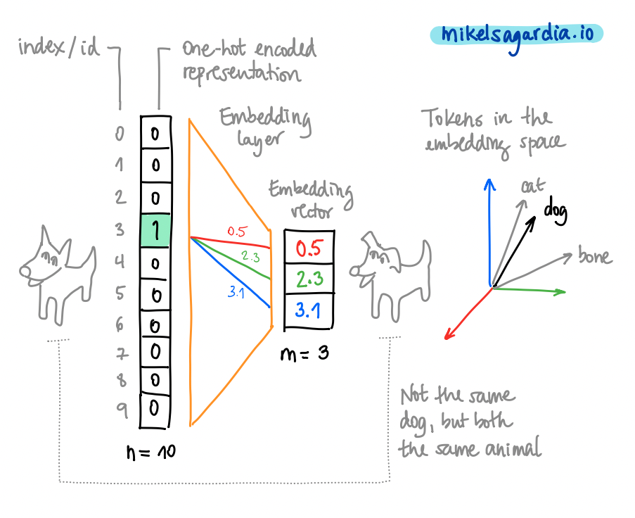
Text vectorization: the word "dog" converted into an embedding vector. Image by the author.

Recurrent Neural Networks

Once we have sequences of vectorized tokens, we can feed them to recursive layers that learn patterns from them. For instance, in our word-wise text generator, we might input a sequence like

The, dog, is, eating, a

and make the model learn to output the target token bone. In other words, the network is trained to predict the likeliest vector(s) given the sequence of vectors we have shown it.

Recursive layers are characterized by the following properties:

• Vectors of each sequence are fed one by one to them.
• Neurons that compose those layers keep a memory state, also known as hidden state.
• The memory state from the previous step, i.e., the one produced by the previous vector in the sequence, is used in the current step to produce a new output and a new memory state.

The most basic recursive layer is the Simple RNN or Elman Network, depicted in the following figure:

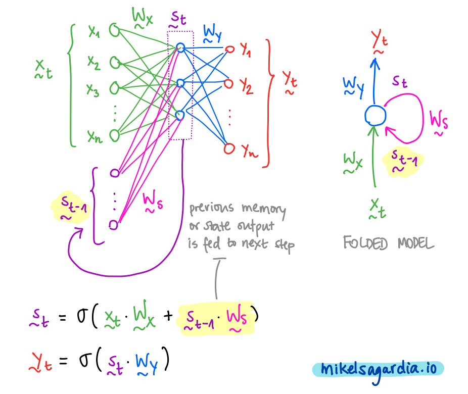
The model of a Simple Recurrent Neural Network or Elman Network. Image by the author.

In the picture, we can see that we have 3 vectors for each time step \(t\): the input \(x\), the output \(y\) and the memory state \(s\). Additionally, the previous memory state is used together with the current input to generate the new memory state, and that new memory state is mapped to be the output. In that process, 3 weight matrices are used (\(W_x\), \(W_y\) and \(W_s\)), which are learned during training.

Unfortunately, simple RNNs or Elman networks suffer from the vanishing gradient problem; due to that, in practice, they can reuse only 8-10 previous steps. Luckily, Long Short-Term Memory (LSTM) units were introduced by Schmidhuber et al. in 1997. LSTMs efficiently alleviate the vanishing gradient issue and they are able handle +1,000 steps backwards.

LSTM cells are differentiable units that perform several operations every step; those operations decide which information is removed from memory, which kept in it and which used to form an output. They segregate the memory input/output into two types, as shown in the next figure:

• short-term memory, which captures recent inputs and outputs,
• and long-term memory, which captures the context.

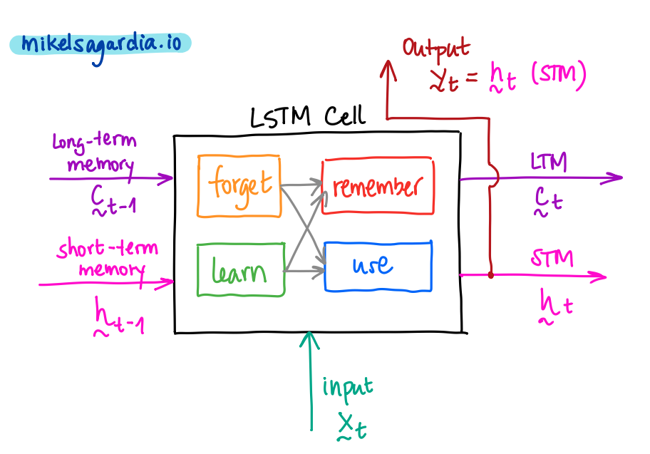
The abstract model of Long Short-Term Memory (LSTM) unit. Image by the author.

Therefore, we have:

• Three inputs:
  • signal/event: \(x_t\)
  • previous short-term memory: \(h_{t-1}\)
  • previous long-term memory : \(C_{t-1}\)
• Three outputs:
  • transformed signal or output: \(y_t = h_t\)
  • current/updated short-term memory: \(h_t\)
  • current/updated long-term memory: \(C_t\)

Note that the updated short-term memory is the signal output, too!

All 3 inputs are used in the cell in 4 different and interconnected gates to generate the 3 outputs; these internal gates are:

• The forget gate, where useless parts of the previous long-term memory are forgotten, creating a lighter long-term memory.
• The learn gate, where the previous short-term memory and the current event are learned.
• The remember gate, in which we mix the light long-term memory with forgotten parts and the learned information to form the new long-term memory.
• The use gate, in which, similarly, we mix the light long-term memory with forgotten parts and the learned information to form the new short-term memory.

If you are interested in more detailed information, Christopher Olah has a great post which explains what’s exactly happening inside an LSTM unit: Understanding LSTM Networks. Also, note that a simpler but similarly efficient alternative to LSTM cells are Gated Recurrent Units (GRUs).

From a pragmatic point of view, it suffices to know that LSTM units have short- and long-term memory vectors which are automatically passed from the previous to the current step. Additionally, the output of the cell is the short-term memory or hidden state, and since we input a sequence of embedded vectors to the unit, we obtain a sequence of hidden vectors.

Final Mapping and Putting It All Together

Usually, 2-3 RNN layers are stacked one after the other and the final output vector sequence can be mapped to the desired target space. For instance, in the case of the text generation example, I have used a fully connected layer which transforms the last vector from the output sequence to one vector of the size of the vocabulary; thus, given a sequence of words/tokens, the model is fit to predict the next most likely one.

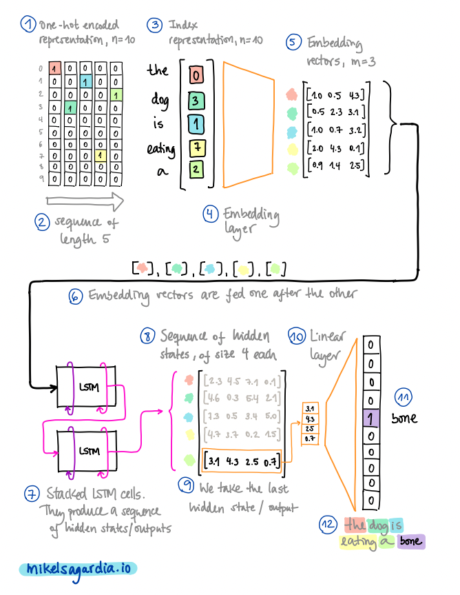
A complete text generation pipeline. In the example, the vocabulary size is n = 10 and we pass a sequence of 5 tokens to the network. The embedding size is m = 3 and the hidden states have a size of 4. Image by the author.

As already mentioned, the output of an LSTM cell is a sequence of hidden states; the length of that sequence is the same as the length of the input sequence and each vector has the size of a hidden state, which can be different than the embedding dimension m (that hidden dimension is a hyperparameter we can modify). Since in our application we only take the last hidden state from that sequence, the defined RNN architecture is of the type many-to-one. However, other types of architectures can be designed thanks to the sequential nature of the RNNs; for instance, we can implement a many-to-many mapping, which is used to perform language translation, or one-to-many, employed in image captioning.

At the end of the day, we need to get the proper dataset we’d like to fit, apply the matrix mappings that match the input features with the target values and learn by optimization the weights within those matrices. Well, with RNNs, we need to consider additionally that we work with sequences.

After seeing a sequence of tokens, the trained model is able to infer the likelihood of each token in the vocabulary to be the next one. That functionality is wrapped in a text generation application that works as follows:

1. We define an initial sequence filled with the padding token and allocate in its last cell a priming word/token. The padding token is a placeholder or empty symbol, whereas the priming token is the seed with which the model will start to generate text.
2. The sequence is fed to the network and it produces the probabilities for all possible tokens. We take a random token from the 5 most likely ones: that is the first generated token/word.
3. The previous input sequence is rolled one element to the front and the last generated token is inserted in the last position.
4. We repeat steps 2 and 3 until we generate the number of words we want.

Results

To train the network, I used the Seinfeld Chronicles Dataset from Kaggle, which contains the complete scripts from the Seinfeld TV Show. To be honest, I’ve never watched Seinfeld, but the conversation does seem to look structurally fine :sweat_smile:

You can judge it by yourself:

jerry: you know, it's the way i can do. i don't know what the hell happened.

jerry: what?

george: what about it?

elaine: i think you could be able to get out of here.

jerry: oh, i can't do anything about the guy.

jerry: what?

george:(smiling) yeah..........

george: you know, you should do the same thing.

jerry: i think i can.

jerry: oh, no, no! no. no.

jerry: i don't know.(to the phone) what do you think?

george: what?

jerry: oh, i think you're not a good friend.

jerry: yeah.

jerry: oh, you can't.

jerry:(to the phone) hey, hey, hey!

jerry:(to jerry) hey hey hey, hey!

george: hey, i can't believe i was gonna have to do that.

george: i don't know how much this is.

kramer:(smiling to jerry) i don't know, i'm not gonna get it.

kramer:(pointing) oh!(starts maniacally pleased to himself, and exits) oh, my god, i don't know!

elaine:(pause) i can't believe i can't. i don't know how much i mean, i was just thinking about this thing! i mean, i'm gonna take it.

george: you know what you want?

elaine: oh yeah, well, i'm gonna go see the way to get it.

elaine: oh yeah, well, i am not gonna get a little uncomfortable for the.

george: what?

george: oh. i don't know what the problem is.

george:(smiling, to himself, he looks in his head.

george: i can't believe you said it was an accident.

elaine: yeah, but you should take some more

Conclusions

In this blog post I explain how the toy word-wise text generator I implemented works. The application uses Recurrent Neural Networks (RNNs) consisting of Long Short-Term Memory (LSTM) units; the parts and steps developed for it are common to many Natural Language Processing (NLP) applications, such as sentiment analysis or image captioning, and I try to answer the central questions around them:

• Text processing: what tokenization and vocabulary generation are, and why we need to vectorize words in embedding spaces.
• RNNs and LSTM units: what these recurrent layers do and the shape of their inputs and outputs.
• Final sequence mapping: how the outputs from recurrent layers can be transformed into the target space.

I trained the model with the Seinfeld Chronicles Dataset from Kaggle and, although the generated text doesn’t make complete sense, the dialogues seem structurally similar to the ones in the dataset; in some cases, I read 1-3 sentences and I can almost hear the sitcom laugh track in the background :joy:

Which text would you like to capture and regenerate?

If you’re interested in more technical details related to the topic, you can have a look at Github repository of the project. Also, if you’d like to see how a very similar architecture as the one used here can be employed to generate text descriptions of image contents, you can have a look at my image captioning project.

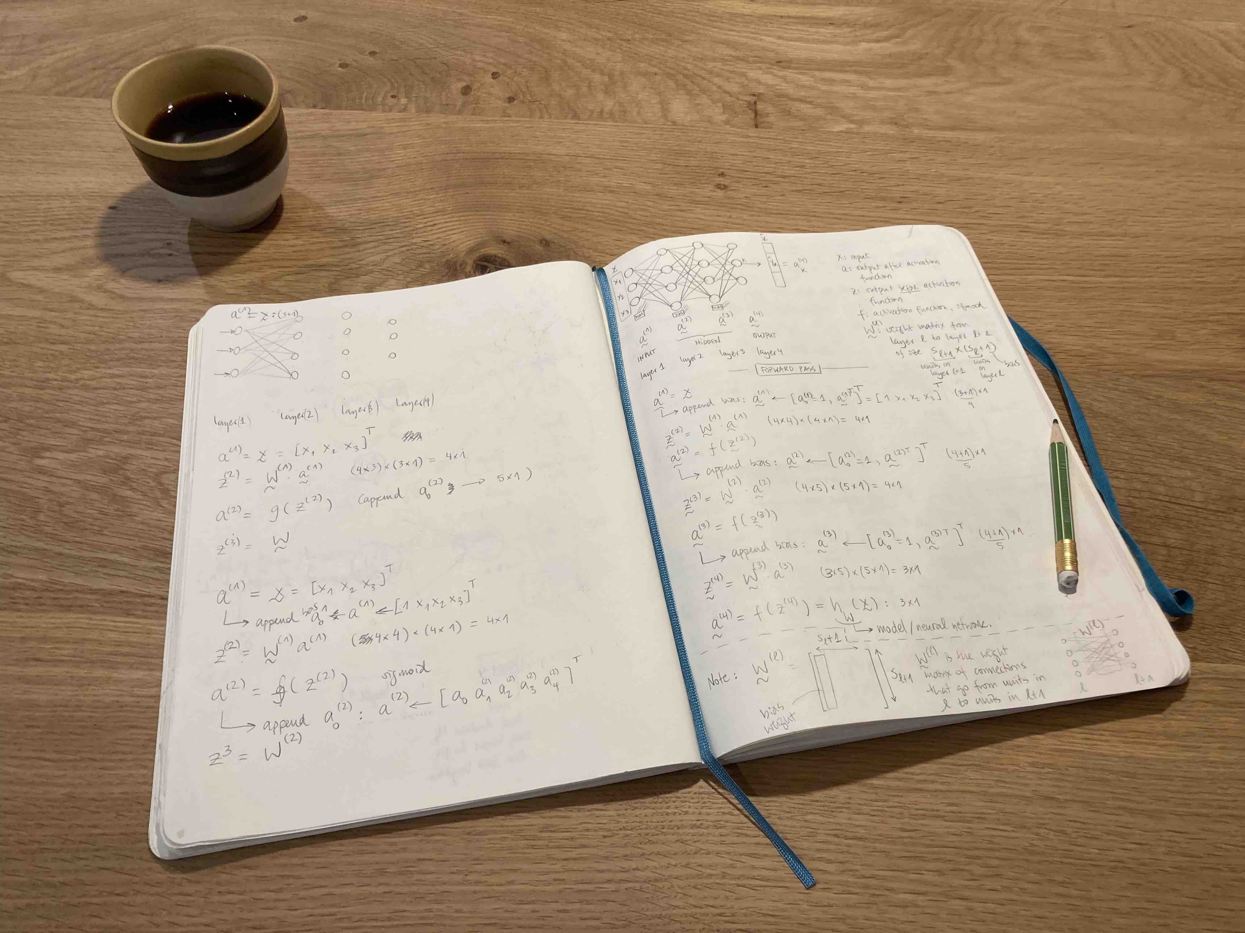
A glimpse to my current notebook. Photo by the author.

I love writing and drawing on my notebook. In there, you’ll find not only formulas or flow charts, but also funny cartoons, interminable lists of things I’d like to do, shopping lists, or important scribbles my kids leave me every now and then. Therefore, one could say they are a unique window to what’s going on in my mind and life.

I think something similar happens with the Jupyter notebooks commonly used in data science: they are great because it’s very easy to try new ideas with code in them, you jot down notes beside the features you engineered or the models you tried, and everything is visually great – but the produced content often grows chaotically and it ends up being unusable in real life without proper modifications.

Photo by SJ on Unsplash.

I have also noticed that I start becoming more sloppy and lazy when I’m too long around notebooks; it’s like when you tend to leave your vegetables unfinished and indulge yourself with cookies for dessert. And then, you try to fit in that wedding suit and you realize it somehow shrunk.

Jupyter Notebooks are like chocolate cookies: You know you should eat them in moderation, but you can’t help sneaking the last one again.

Applying Software Engineering and DevOps to Research Code

Food metaphores aside, and using the jargon of the Software Engineering world, Jupyter notebooks belong to research and development environments, whereas deployed code belongs to production environments. Most of the data science projects don’t leave the research environment, because their goal is to provide useful insights. However, when the created models need to be used in online predictions with new data, we need to level up the code and the infrastructure quality to meet the production standards, characterized by a guarantee of reliability.

Machine learning systems have particular properties that present new challenges in production, as Sculley et al. pointed out in their motivational foundations of what is becoming the field of MLOps. Many tools which target those specific needs have appeared in recent years; those tools and the applications which use them are often categorized in maturity levels:

• Level 0 (research and development): data analysis and modeling is performed to answer business questions, but the models are not used to perform online inferences.
• Level 1 (production): the inference pipeline is deployed manually and the artifact versions are tracked (models, data, code, etc.) and pipeline outputs monitored.
• Level 2 (very serious production): deployments of training and inference pipelines are done automatically and frequently, enabling large-scale continuously updated applications.

Small/medium-sized projects (teams of 1-20 people) require typically level 1 maturity, and often, the companies where they are implemented in don’t have the resources to go for level 2.

In this article, I present a standardized way of transforming research notebooks into production-level code; in MLOps maturity levels that represents the journey from level 0 to 1. To that end, I have implemented a boilerplate project with production-ready quality that can be cloned from this Github repository.

The selected business case consists in analyzing customer churn using the Credit Card Customers dataset from Kaggle. Data analysis, modeling and inference pipelines are implemented in the project to end up with an interpretable model-pipeline that is also able to perform reliable predictions. However, the package is designed so that the business case and the data analysis can be easily replaced, and the focus lies in providing a template with the following properties:

• Structure which reflects the typical steps in a small/medium-sized data science project
• Readable, simple, concise code
• PEP8 conventions applied, checked with pylint and autopep8
• Modular and efficient code, with Object-Oriented patterns
• Documentation provided at different stages: code, README files, etc.
• Error/exception handling
• Execution and data testing with pytest
• Logging implemented during production execution and testing
• Dependencies controlled for custom environments
• Installable python package
• Basic containerization with Docker

However, two properties are missing to reach full level 1:

• Deployment of the pipeline
• Tracking of the generated artifacts (model-pipelines, data, etc.)
• Monitoring of the model (drift)

Those are fundamental attributes, but I consider they are out of scope in this article/project, because they often rely on additional 3rd party tools. My goal is to provide a template to transform notebook code into professional software using the minimum additional tools it is possible; after that, we have a solid base to add more layers that take care of the tracking and monitoring of the different elements.

The Boilerplate

The boilerplate project from the Github repository has the following basic file structure:

.
├── README.md                         # Package description, usage, etc.
├── churn_notebook.ipynb              # Research notebook
├── config.yaml                       # Configuration file for production
├── customer_churn/                   # Production library, package
│   ├── __init__.py                   # Python package file         
│   ├── churn_library.py              # Production library
│   └── transformations.py            # Utilities for the library
├── data/                             # Dataset folder
│   ├── README.md                     # Dataset details
│   └── bank_data.csv                 # Dataset file
├── main.py                           # Executable of production code
├── requirements.txt                  # Dependencies
├── setup.py                          # Python package file
└── tests/                            # Pytest testing scripts
    ├── __init__.py                   # Python package file
    ├── conftest.py                   # Pytest fixtures
    └── test_churn_library.py         # Tests for churn_library.py

All the research work of the project is contained in the notebook churn_notebook.ipynb; in particular, simplified implementations of the typical data processing and modeling tasks are performed:

1. Data Acquisition/Import
2. Exploratory Data Analysis (EDA)
3. Data Processing: Data Cleaning, Feature Engineering (FE)
4. Data Modelling: Training, Evaluation, Interpretation
5. Model Scoring: Inference

The code from churn_notebook.ipynb has been transformed to create the package customer_churn, which contains two files:

• churn_library.py: this file contains most of the refactored and modified code from the notebook.
• transformations.py: definition of auxiliary transformations used in the data processing; complex operations on the data are implemented in Object-Oriented style so that they can be cleanly applied as with the sklearn.preprocessing package.

Additionally, a tests folder is provided, which contains test_churn_library.py. This script performs unit tests on the different functions of churn_library.py using pytest.

The executable or main function is provided in main.py; this script imports the package customer_churn and runs three functions from churn_library.py:

• run_setup(): the configuration file config.yaml is loaded and auxiliary folders are created, if not there yet:
  • images: it will contain the images of the EDA and the model evaluation.
  • models: it will contain the inference models/pipelines as serialized objects (pickles).
  • artifacts: it will contain the data processing parameters created during the training and required for the inference, serialized as pickles.
• run_training(): it performs the EDA, the data checks, the data processing and modeling, and it generates the inference artifacts (the model/pipeline), which are persisted as serialized objects (pickles). In the provided example, logistic regression, support vector machines and random forests are optimized in a grid search to find the best set of hyperparameters.
• run_inference(): it shows how the inference artifacts need to be used to perform a prediction; an exemplary dataset sample created during the training is used.

The following diagram shows the workflow:

Although the training and the inference pipeline represented by run_training() and run_inference() should run sequentially one after the other, the symmetry of both is clear; in fact, a central property of the package is that run_training() and run_inference() share the function perform_data_processing(). When perform_data_processing() is executed in run_training(), it generates the processing parameters and stores them to disk. In contrast, when perform_data_processing() is executed in run_inference(), it loads those stored parameters to perform the data processing for the inference.

Note that the implemented run_inference() is exemplary and it needs to be adapted:

• Currently, it is triggered manually and it scores a sample dataset from a CSV file offline; instead, we should wait for external requests that feed new data to be scored.
• The data processing parameters and the model should be loaded once in the beginning (hence, the dashed box) and used every time new data is scored.

Those intentional loose ends are to be tied when deciding how to deploy the model, which is not in the scope of this repository, as mentioned.

Finally, note that this boilerplate is designed for small/medium datasets, which are not that uncommon in small/medium enterprises; in my experience, its structure is easy to understand, implement and adapt. However, as the complexity increases (e.g., when we need to apply extensive feature engineering), it is recommended to apply these changes to the architecture:

• All data processing steps should be written in an Object Oriented style and packed into a Scikit-Learn Pipeline (or similar), as done in transformations.py.
• Any data processing that must be applied to new data should be integrated in the inference pipeline generated in train_models(); that means that we should integrate most of the content in perform_data_processing() as a Pipeline in train_models(). Thus, perform_data_processing() would be reduced to basic tasks related to cleaning (e.g., duplicate removal) and checking.

More details on the package can be found on the source Github repository.

Conclusions

In this article I introduced my personal boilerplate to transform small/medium-sized data science projects into production-ready packages without exposing to many 3rd party tools. The template works on the customer churn prediction problem using the Credit Card Customers dataset from Kaggle, but you are free to clone the boilerplate from its Github repository and modify it for your business case. Important software engineering aspects as covered, such as, clean code conventions, modularity, reproducibility, logging, error and exception handling, testing, dependency handling with environments – and more.

Topics such as data processing techniques, pipeline deployment, artifact tracking and model monitoring are out of scope; for them, have a look at the following links:

• A 80/20 Guide for Exploratory Data Analysis, Data Cleaning and Feature Engineering.
• A Boilerplate for Reproducible and Tracked Machine Learning Pipelines with MLflow and Weights & Biases and Its Application to Song Genre Classification.
• Deployment of a Census Salary Classification Model Using FastAPI.
• If you are interested in more MLOps-related content, you can visit my notes on the Udacity Machine Learning DevOps Engineering Nanodegree: mlops_udacity.

Do you find the boilerplate helpful? What would you add or modify? Do you know similar templates to learn from?

Don't worry, working hard often pays off. Photo by Tim Gouw on Unsplash.

Thanks to the powerful packages we have available nowadays, training machine learning models is often a very tiny step in the pipeline of a regular data science project. Altogether, we need to address the following tasks:

1. Data Understanding & Formulation of the Questions
2. Data Cleaning
3. Exploratory Data Analysis
4. Feature Engineering
5. Feature Selection
6. Data Modelling

Additionally, if online inferences are planned, several parts from the steps 2-5 needs to be prepared for production environments, i.e., they need to be transferred into scripts in which reproducibility and maintainability can be guaranteed for robust and trustworthy deployments.

Independently from that fact and remaining still in the research and development environment, steps 2-5 consume a large percentage of the effort. We need to apply some kind of methodical creativity to often messy datasets that almost never behave as we initially want.

So, is there an easy way out? Unfortunately, I’d say there is not, at least I don’t know one yet. However, I have collected a series of guidelines and code snippets you can use systematically to ease your data processing journey in a Github repository. It summarizes the map I have sketched along the years.

In the repository, you will find two important files:

• A large python script data_processing.py which contains many code examples; these cover 80% of the processing techniques I usually apply on tabular datasets.
• The README.md itself, which sums up the steps and dos & don’ts in the standard order for data processing described above.

Some caveats:

• The script data_processing.py does not run! Instead, it’s a compilation of useful commands with comments.
• I assume the reader knows the topic, i.e., the repository is not for complete beginners.
• The guide does not cover advanced cases either: it’s a set of tools that follow the 80/20 Pareto principle.
• The guide focuses on tabular data; images and text have their own particular pipelines, not covered here.
• This is my personal guide, made for me; no guarantees are assured and it will probably change organically.

Do you find the repository helpful? What would you add? Do you know similar summaries to learn from?

Donostia-San Sebastian. Photo by @ultrashricco from Unsplash.

In 2020 I decided to move back to my birthplace in the Basque Country (Spain) after almost 15 years in Munich (Germany). The Basque region in Spain is a popular touristic destination, as it has a beautiful seaside with a plethora of surfing spots and alluring hills that call for hiking and climbing adventures. Culture and gastronomy are also important features, both embedded in a friendly and developed society with modern infrastructure.

When the pandemic seemed to start fading away in spring 2022, friends and acquaintances from Europe began asking me about the best areas and trips in the region, hotels and hostels to stay in case there was no room in my place, etc. The truth is, after so many years abroad I was not the best person to guide them with updated information; however, the AirBnB dataset from Euskadi (i.e., Basque Country in Basque language) has clarified some of my questions. The dataset contains, among others, a list of 5228 accommodations, each one of them with 74 variables.

Following the standard CRISP-DM process for data analysis, I have cleaned, processed and modelled the dataset to answer three major business questions:

1. Prices. Is it possible to build a model that predicts the price from the variables? If so, which are the most important variables that determine the price? Can we detect accommodations that, having a good review score, are a bargain?
2. Differences between accommodations with and without beach access. Surfing or simply enjoying the seaside are probably some important attractions visitors seek on their vacations. However, not all accommodations are a walk distance from a beach. How does that influence the features of the housings?
3. Differences between the two most important cities: Donostia-San Sebastian and Bilbao. These province capitals are the biggest and most visited cities in the Basque Country; in fact, their listings account for 50% of all offered accommodations. However, both cities are said to have a different character: Bilbao is a bigger, modern city, without beach access but probably with richer cultural offerings and nightlife; meanwhile, Donostia-San Sebastian is more aesthetic, it has three beaches and it’s perfect for day-strolling. How are those popular differences reflected on the features of the accommodations?

The Dataset

AirBnB provides with several CSV files for each world region: (1) a listing of properties that offer accommodation, (2) reviews related to the listings, (3) a calendar and (4) geographical data. A detailed description of the features in each file can be found in the official dataset dictionary.

My analysis has concentrated on the listings file, which consists in a table of 5228 rows/entries (i.e., the accommodation places) and 74 columns/features (their attributes). Among the features, we find continuous variables, such as:

• the price of the complete accommodation,
• accommodates: maximum number of persons that can be accommodated,
• review scores for different dimensions,
• reviews per month,
• longitude and latitude,
• etc.

… categorical variables:

• neighbourhood name,
• property type (apartment, room, hotel, etc.)
• licenses owned by the host,
• amenities offered in the accommodation,
• etc.

… date-related data:

• first and last review dates,
• date when the host joined the platform,

… and image and text data:

• URL of the listing,
• URL of the pictures,
• description of the listing,
• etc.

Of course, not all features are meaningful to answer the posed questions. The explanations given on my Gihub repository describe in detail how I dealt with noisy and missing values, and how some features were dropped or some other engineered. After that processing, we get a new table with 3931 entries and 353 features.

So… Would like to have a look at what I have learned from the data? Let’s dive in!

Question 1: Prices

In order check whether we can predict the price, I have trained several models with 90% of the processed dataset (i.e., the training split) using Scikit-Learn: (1) linear regression as baseline, (2) Ridge regression (L2 regularized regression), (3) Lasso regression (L1 regularized regression) and (2) random forests. Cross-validation was performed with all of them and their hyperparameters were tuned; additionally, the effect of polynomial features on the model performances was also studied, as thoroughly summarized on the Gihub repository.

The modelling experiments show that the random forests model seems to score the best R2 value for the test split: 69% of the variance can be explained with the random decision trees. Moreover, adding polynomial terms does not improve predictions for the present dataset. The following diagram shows the performance of the Ridge regression model and the random forests model with the test split using only the 353 linear features.

The models tend to under-predict accommodation prices; that bias clearly increases as the prices start to be larger than 50 USD. Such a moderate R2 is not the best one to apply the model to perform predictions. However, we can deduce the most important features that determine the listing prices if we compute the Gini importances, as done in the following diagram. The top-5 variables that determine the price of a listing are:

• whether an accommodation is an entire home or apartment,
• the number of bathrooms in it,
• the number of accommodates,
• whether the bathroom(s) is/are shared,
• and whether the housing is located in Donostia-San Sebastian.

Note that only the top-30 features are shown; these account for almost 89% of the accumulated Gini importance (all 353 variables would account for 100%).

But how does increasing the value of each feature affect the price: does it contribute to an increase in price or a decrease? That can be observed in the following diagram, similar to the previous one. In contrast to the former, here the 30 regression coefficients with the largest magnitude are plotted - red bars are associated with features that decrease the price when they are increased, i.e., negative coefficients.

Being different models, different features appear in the ranking; in any case, both lists are consistent and provide valuable insights. For instance, we deduce that the price decreases the most when

• the number of reviews per month increases (note that review positivity is not measured),
• the host is estimated to have shared rooms,
• the accommodation is a shared room,
• and when the bathroom(s) is/are shared.

Finally, a very practical insight to close the pricing question: we can easily select the the accommodations which have a very good average review (above the 90% percentile) and yield a model price larger than the real one, as shown in the following figure. These are the likely bargains!

I prefer not post the URLs of the detected listings, but it is straightforward to obtain them using the notebooks of the linked repository :wink:.

Question 2: To Beach or not to Beach

Of course, you can always go to the beach to catch some waves in the Basque Country, but going on foot and in less than 15 minutes has an additional cost, on average. That is one of the insights distilled from the next diagram.

This difference or significance plot shows the T and Z statistics computed for each feature considering two independent groups: accommodations with and without beach access. These statistics are related to the difference of means (T statistic, for continuous variables) or proportions (Z statistic, for discrete variables or proportions). If we take the usual significance level of 5%, the critical Z or T value is roughly 2. That means that if the values in the diagram are greater than 2, the averages or proportions of each group in each feature are significantly different. The probability of being otherwise but incorrectly stating that they are different is 5%.

The sign of the statistic is color-coded: blue bars denote positive statistics, which are associated with larger values for accommodations that have beach access.

Long story short, here’s the interpretation: the group of accommodations that have a beach within 2 km have significantly larger

• proportions of accommodations located in the province of Gipuzkoa, compared to Bizkaia,
• proportions of accommodations with a waterfront,
• and prices.

Note that larger statistics don’t necessarily mean larger differences; instead, they mean that the probability of wrongly stating a difference between groups is lower.

Instead of reading the ranking top-down, it is more interesting to compose a profile of listings with beach access and without by selecting features manually; for instance, the accommodations on the seaside:

• have larger prices,
• are more often entire homes or apartments,
• usually have less shared bathrooms,
• have more often a description in English instead of in Spanish (i.e., they target more foreign tourists),
• have more often a beachfront, patio or balcony,
• have more bedrooms,
• allow for more accommodates but for longer minimum periods,
• their host lives more often nearby,
• …

Going back to the price, the following figure shows the different price distributions for accommodations with a beach in less than 2 km and further. We need to consider that there is such a distribution or a contingency table behind each of the Z/T statistics in the previous diagram.

Question 3: Athletic de Bilbao vs. Real Sociedad

If you’re a soccer fan, maybe you’ve heard about the Basque derby: Athletic de Bilbao vs. Real Sociedad. Both football teams are originally from the two major cities in the Basque Country, Bilbao and Donostia-San Sebastian, and they represent the healthy rivalry between the two province capitals.

In order to determine the differences between the two cities in terms of listing features, I have computed the same difference or significance plot as before, shown below.

Donostia-San Sebastian seems to have

• larger prices,
• more accommodations with waterfronts,
• more descriptions in English,
• hosts that joined AirBnB longer ago and who have more accommodations,
• more often patios or balconies,
• more often entire homes or apartments,
• more space for accommodates,
• …

On the other hand, Bilbao has

• more accommodations that are a bedroom,
• more shared bathrooms,
• more amenities, such as shampoo, hangers, first aid kits, extra pillows, breakfast
• …

Finally, as before, I leave the price distribution for both cities, since it is the feature in which the difference is more significant. We can see that the distribution from Bilbao has more units in the lowest price region, whereas the red city lacks listings with prices above 150 USD, compared to Donostia-San Sebastian. That is in line with several already explained facts, such as that Bilbao has more shared rooms, whereas Donostia has more entire homes, while being the effect on the price of both characteristics the opposite.

Conclusions

In this blog post, we took a look at the AirBnB accommodation properties from the Basque Country, narrowing down to these insights:

1. Even though the price regression models have a moderate R2, we have shown how to detect listings which are candidate to be a bargain: accommodations with high review scores and predicted price above the true one. Additionally, we have discovered the features with the largest impact on the price: type of accommodation, bathrooms, locations, etc.
2. Listings with a beach in less than 2 km have significantly more entire homes, more balconies, waterfronts and space for more accommodates; this is in line with their larger prices.
3. The two major cities Donostia-San Sebastian and Bilbao nicely align with the previous synthesis, being Donostia a beach city and Bilbao a city without. Additionally, Bilbao seems to favor other practical domestic amenities.

These conclusions are quite informal, but I hope they can guide my data-savvy friends; in any case, I’m sure you can have a great vacation anywhere you go in the Basque Country :)

Are you planning a trip to the Basque Country? Has this blog post helped you?

To learn more about this analysis, see the link to my Gihub repository. You can download the pre-processed dataset and ask the data your own specific questions!