A Toy Recurrent Neural Network Based on LSTM Cells Which Generates TV Scripts

A chimpanzee seated at a typewriter "If you give me an infinite number of bananas I'll type banana for you." Photo from Wikimedia.

The infinite monkey theorem states that a monkey writing random letters on a keyboard long enough can reproduce the complete works of Shakespeare. There is even a straightforward proof when long enough tends to infinity.

Now, I don’t plan to have monkeys in my cellar and I surely don’t have infinite time. But could maybe neural networks aid in that enterprise? It turns out, they can, and they are astonishingly effective even with small tweaking efforts.

Deep neural networks are amazingly good at learning patterns and one can take advantage of that to generate new and structurally coherent data.

Inspired by the great post from Andrej Karpathy in which he describes how text can be generated character-wise, I implemented a word-wise text generator which works with Recurrent Neural Networks (RNNs). My code can be found in this Github repository.

Are you interested in how this is possible? Let’s dive in!

Recursive Neural Networks and Their Application to Language Modeling

While Convolutional Neural Networks (CNNs) are particularly good at capturing spatial relationships, Recurrent Neural Networks (RNNs) model sequential structures very efficiently. Also, in recent years, the Transformer architecture has been shown to work remarkably well with language data – but let’s keep it aside for this small toy project.

In many language modeling applications, and in the particular text generation case explained here, we need to undertake the following general steps:

The text needs to be processed as sequences of numerical vectors.
We define recurrent layers which take those sequences of vectors and yield sequences of outputs.
We take the complete or partial output sequence and we map it to the target space, e.g., words.

Let’s analyze in more detail what happens in each step.

Text Preprocessing

Computers are able to work only with numbers. The same way an image is represented as a matrix of pixels that contain R-G-B values, sentences need to be transformed into numerical values. One common recipe to achieving that is the following:

The text is tokenized: it is converted into a list of elements or tokens that have an identifiable unique meaning; these elements are usually words and related symbols, such as question marks or other punctuation elements.
A vocabulary is created: we generate a dictionary with all the n unique tokens in the dataset which maps from the token string to an id and vice versa.
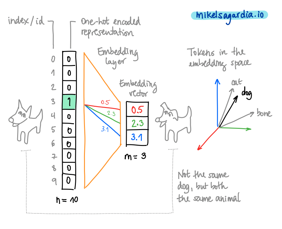
Tokens are vectorized: tokens can be represented as one-hot encoded vectors, i.e., each of them becomes a vector of size n which contains all 0-s except in the index/cell which corresponds to the token id in the vocabulary, where the value 1 is assigned. Then, those one-hot encoded vectors can be compressed to an embedding space consisting of vectors of size m, with m << n. Those embedded vectors contain floating point numbers, i.e., they are not sparse as their one-hot encoded version. That mapping is achieved with an embedding layer, which is akin to a linear layer, and it considerably improves the model efficiency. Typical reference sizes are n = 70,000, m = 300.

Note that, in practice, one-hot encoding the tokens can be skipped. Instead, tokens are represented with their id or index values in the vocabulary and the embedding layer handles everything with that information. That is possible because each token has a unique id value which triggers m unique weights only. The following figure illustrates that idea and the overall vectorization of the tokens:

Text vectorization: the word 'dog' converted into an embedding vector
Text vectorization: the word "dog" converted into an embedding vector. Image by the author.

Recurrent Neural Networks

Once we have sequences of vectorized tokens, we can feed them to recursive layers that learn patterns from them. For instance, in our word-wise text generator, we might input a sequence like

The, dog, is, eating, a

and make the model learn to output the target token bone. In other words, the network is trained to predict the likeliest vector(s) given the sequence of vectors we have shown it.

Recursive layers are characterized by the following properties:

Vectors of each sequence are fed one by one to them.
Neurons that compose those layers keep a memory state, also known as hidden state.
The memory state from the previous step, i.e., the one produced by the previous vector in the sequence, is used in the current step to produce a new output and a new memory state.

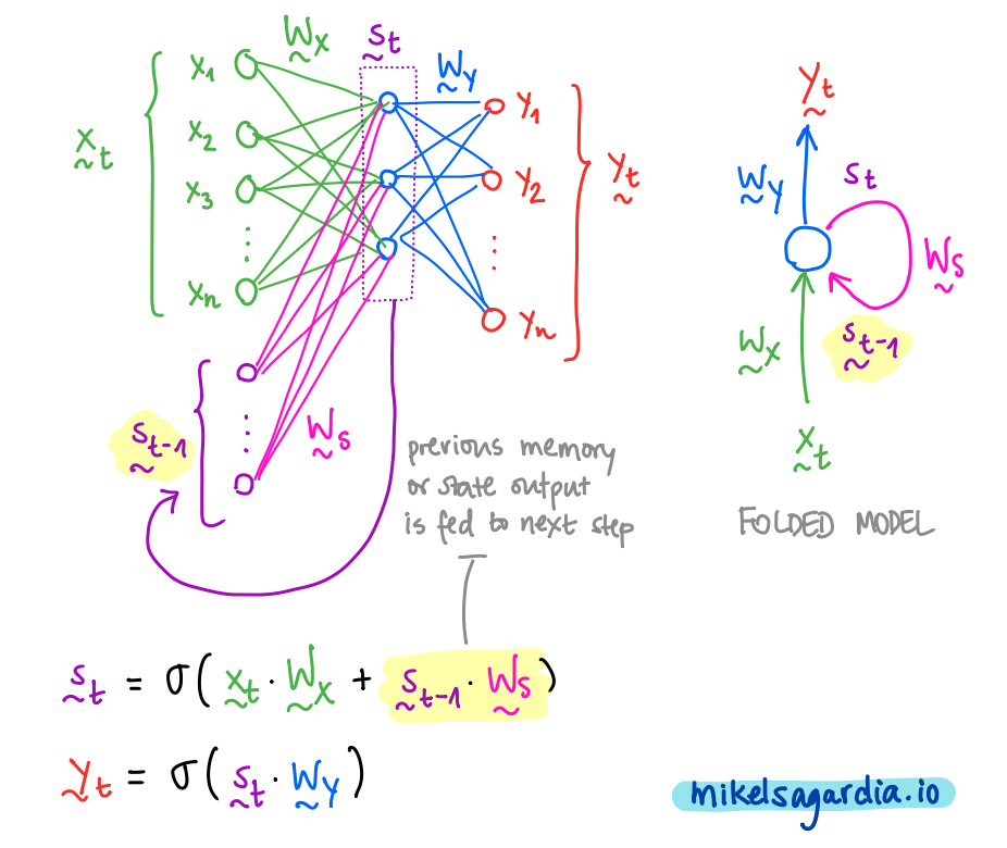
The most basic recursive layer is the Simple RNN or Elman Network, depicted in the following figure:

The model of a Simple Recurrent Neural Network or Elman Network. Image by the author.

In the picture, we can see that we have 3 vectors for each time step \(t\): the input \(x\), the output \(y\) and the memory state \(s\). Additionally, the previous memory state is used together with the current input to generate the new memory state, and that new memory state is mapped to be the output. In that process, 3 weight matrices are used (\(W_x\), \(W_y\) and \(W_s\)), which are learned during training.

Unfortunately, simple RNNs or Elman networks suffer from the vanishing gradient problem; due to that, in practice, they can reuse only 8-10 previous steps. Luckily, Long Short-Term Memory (LSTM) units were introduced by Schmidhuber et al. in 1997. LSTMs efficiently alleviate the vanishing gradient issue and they are able handle +1,000 steps backwards.

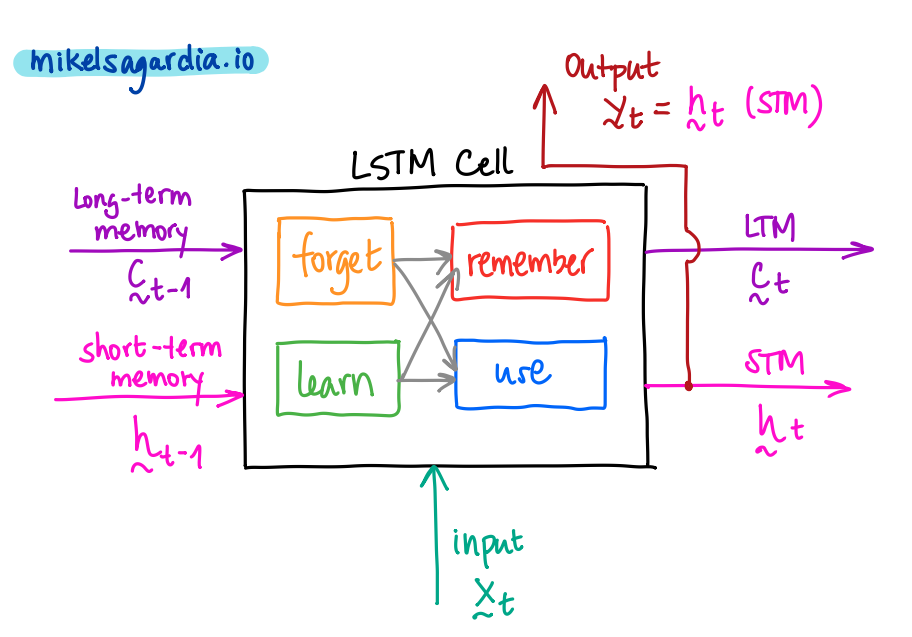
LSTM cells are differentiable units that perform several operations every step; those operations decide which information is removed from memory, which kept in it and which used to form an output. They segregate the memory input/output into two types, as shown in the next figure:

short-term memory, which captures recent inputs and outputs,
and long-term memory, which captures the context.

The abstract model of Long Short-Term Memory (LSTM) unit. Image by the author.

Therefore, we have:

Three inputs:
- signal/event: \(x_t\)
- previous short-term memory: \(h_{t-1}\)
- previous long-term memory : \(C_{t-1}\)
Three outputs:
- transformed signal or output: \(y_t = h_t\)
- current/updated short-term memory: \(h_t\)
- current/updated long-term memory: \(C_t\)

Note that the updated short-term memory is the signal output, too!

All 3 inputs are used in the cell in 4 different and interconnected gates to generate the 3 outputs; these internal gates are:

The forget gate, where useless parts of the previous long-term memory are forgotten, creating a lighter long-term memory.
The learn gate, where the previous short-term memory and the current event are learned.
The remember gate, in which we mix the light long-term memory with forgotten parts and the learned information to form the new long-term memory.
The use gate, in which, similarly, we mix the light long-term memory with forgotten parts and the learned information to form the new short-term memory.

If you are interested in more detailed information, Christopher Olah has a great post which explains what’s exactly happening inside an LSTM unit: Understanding LSTM Networks. Also, note that a simpler but similarly efficient alternative to LSTM cells are Gated Recurrent Units (GRUs).

From a pragmatic point of view, it suffices to know that LSTM units have short- and long-term memory vectors which are automatically passed from the previous to the current step. Additionally, the output of the cell is the short-term memory or hidden state, and since we input a sequence of embedded vectors to the unit, we obtain a sequence of hidden vectors.

Final Mapping and Putting It All Together

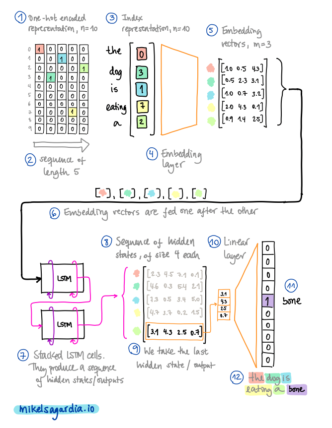
Usually, 2-3 RNN layers are stacked one after the other and the final output vector sequence can be mapped to the desired target space. For instance, in the case of the text generation example, I have used a fully connected layer which transforms the last vector from the output sequence to one vector of the size of the vocabulary; thus, given a sequence of words/tokens, the model is fit to predict the next most likely one.

The complete text generation pipeline
A complete text generation pipeline. In the example, the vocabulary size is n = 10 and we pass a sequence of 5 tokens to the network. The embedding size is m = 3 and the hidden states have a size of 4. Image by the author.

As already mentioned, the output of an LSTM cell is a sequence of hidden states; the length of that sequence is the same as the length of the input sequence and each vector has the size of a hidden state, which can be different than the embedding dimension m (that hidden dimension is a hyperparameter we can modify). Since in our application we only take the last hidden state from that sequence, the defined RNN architecture is of the type many-to-one. However, other types of architectures can be designed thanks to the sequential nature of the RNNs; for instance, we can implement a many-to-many mapping, which is used to perform language translation, or one-to-many, employed in image captioning.

At the end of the day, we need to get the proper dataset we’d like to fit, apply the matrix mappings that match the input features with the target values and learn by optimization the weights within those matrices. Well, with RNNs, we need to consider additionally that we work with sequences.

After seeing a sequence of tokens, the trained model is able to infer the likelihood of each token in the vocabulary to be the next one. That functionality is wrapped in a text generation application that works as follows:

We define an initial sequence filled with the padding token and allocate in its last cell a priming word/token. The padding token is a placeholder or empty symbol, whereas the priming token is the seed with which the model will start to generate text.
The sequence is fed to the network and it produces the probabilities for all possible tokens. We take a random token from the 5 most likely ones: that is the first generated token/word.
The previous input sequence is rolled one element to the front and the last generated token is inserted in the last position.
We repeat steps 2 and 3 until we generate the number of words we want.

Results

To train the network, I used the Seinfeld Chronicles Dataset from Kaggle, which contains the complete scripts from the Seinfeld TV Show. To be honest, I’ve never watched Seinfeld, but the conversation does seem to look structurally fine

You can judge it by yourself:

jerry: you know, it's the way i can do. i don't know what the hell happened.

jerry: what?

george: what about it?

elaine: i think you could be able to get out of here.

jerry: oh, i can't do anything about the guy.

jerry: what?

george:(smiling) yeah..........

george: you know, you should do the same thing.

jerry: i think i can.

jerry: oh, no, no! no. no.

jerry: i don't know.(to the phone) what do you think?

george: what?

jerry: oh, i think you're not a good friend.

jerry: yeah.

jerry: oh, you can't.

jerry:(to the phone) hey, hey, hey!

jerry:(to jerry) hey hey hey, hey!

george: hey, i can't believe i was gonna have to do that.

george: i don't know how much this is.

kramer:(smiling to jerry) i don't know, i'm not gonna get it.

kramer:(pointing) oh!(starts maniacally pleased to himself, and exits) oh, my god, i don't know!

elaine:(pause) i can't believe i can't. i don't know how much i mean, i was just thinking about this thing! i mean, i'm gonna take it.

george: you know what you want?

elaine: oh yeah, well, i'm gonna go see the way to get it.

elaine: oh yeah, well, i am not gonna get a little uncomfortable for the.

george: what?

george: oh. i don't know what the problem is.

george:(smiling, to himself, he looks in his head.

george: i can't believe you said it was an accident.

elaine: yeah, but you should take some more

Conclusions

In this blog post I explain how the toy word-wise text generator I implemented works. The application uses Recurrent Neural Networks (RNNs) consisting of Long Short-Term Memory (LSTM) units; the parts and steps developed for it are common to many Natural Language Processing (NLP) applications, such as sentiment analysis or image captioning, and I try to answer the central questions around them:

Text processing: what tokenization and vocabulary generation are, and why we need to vectorize words in embedding spaces.
RNNs and LSTM units: what these recurrent layers do and the shape of their inputs and outputs.
Final sequence mapping: how the outputs from recurrent layers can be transformed into the target space.

I trained the model with the Seinfeld Chronicles Dataset from Kaggle and, although the generated text doesn’t make complete sense, the dialogues seem structurally similar to the ones in the dataset; in some cases, I read 1-3 sentences and I can almost hear the sitcom laugh track in the background

Which text would you like to capture and regenerate?

If you’re interested in more technical details related to the topic, you can have a look at Github repository of the project. Also, if you’d like to see how a very similar architecture as the one used here can be employed to generate text descriptions of image contents, you can have a look at my image captioning project.