How Are Large Language Models (LLMs) Built?
A Conceptual Guide for Developers & ML Practitioners
 Large Language Models (LLMs) have been called stochastic parrots by some; in any case, they seem to be here to stay — and to be honest, I find them quite useful, if properly used. Image generated using Dall-E 3; prompt: Wide, landscape cartoon illustration of a happy, confident red-blue-yellow macaw wearing black sunglasses, perched on a tree branch in a green forest, with a white comic speech bubble saying "42"
.
Large Language Models (LLMs) have been called stochastic parrots by some; in any case, they seem to be here to stay — and to be honest, I find them quite useful, if properly used. Image generated using Dall-E 3; prompt: Wide, landscape cartoon illustration of a happy, confident red-blue-yellow macaw wearing black sunglasses, perched on a tree branch in a green forest, with a white comic speech bubble saying "42"
.
The release of ChatGPT in November 2022 revolutionized everyday life in much of the developed world. In a similar way that Google convinced us the Internet was truly useful — and that we needed their search engine — or Apple introduced the first genuinely usable smartphone that made the digital world ubiquitous, OpenAI came up with the next logical step: assistant chatbots based on Large Language Models (LLMs). Language models already existed, but OpenAI’s chat-based user interface, combined with the emergent capabilities of their huge models, led to the perfect killer app: an ever-ready genie that seems to confidently know the answer to everything.
It feels like “ask ChatGPT” has become the new “google it”.
Current LLMs are based on the Transformer architecture, introduced by Google in the seminal work Attention Is All You Need (Vaswani et al. 2017). Before that, LSTMs or Long short-term memory networks (Hochreiter & Schmidhuber, 1997) were the state-of-the-art sequence models for Natural Language Processing (NLP). In fact, many of the concepts exploited by the Transformer were developed using LSTMs as the backbone, and one could argue that LSTMs are, in some respects, more sophisticated models than the Transformer itself — if you’d like an example of an LSTM-based language modeler, you can check this TV script generator of mine.
However, the Transformer presented some major practical advantages that enabled a paradigm shift:
- Its self-attention mechanism made it possible to convert inherently sequential tasks into parallelizable ones.
- Its uncomplicated, modular architecture made it easy to scale up and adapt to many different tasks.
Simultaneously, Howard & Ruder (2018) demonstrated that transfer learning worked not only in computer vision, but also for NLP: they showed that a language model pre-trained on a large corpus could be fine-tuned for smaller corpora and other downstream tasks.
And that’s how the way to the current LLMs was paved. Nowadays, Transformer-based LLMs excel in everything NLP-related: text generation, summarization, question answering, code generation, translation, and so on.
The Original Transformer: Its Inputs, Components and Siblings
Before describing the components of the Transformer, we need to explain how text is represented for computers. In practice, text is converted into a sequence of feature vectors ${x_1, x_2, …}$, each of dimension $m$ (the embedding size or dimension). This is done in the following steps:
- Tokenization: The text is split into discrete elements called tokens. Tokens are units with an identifiable meaning for the model and typically include words or sub-words, as well as punctuation and special symbols.
- Vocabulary construction: A vocabulary containing all $n$ unique tokens is defined. It provides a mapping between each token string and a numerical identifier (token ID).
- One-hot vectors: Each token is mapped to its token ID. Conceptually, this corresponds to a one-hot vector of size $n$, although in practice models operate directly on token IDs. In a one-hot vector, all cells have the value $0$ except the cell which corresponds to the token ID of the represented word, which contains the value $1$.
- Embedding vectors: Token IDs (i.e., one-hot vectors) are mapped to dense embedding vectors using an embedding layer. This layer acts as a learnable lookup table (or equivalently, a linear projection of a one-hot vector), producing vectors of size $m$, with $m \ll n$. These embedding vectors are simply arrays of floating-point values. Typical reference values are $n \approx 100{,}000$ and $m \approx 500$.
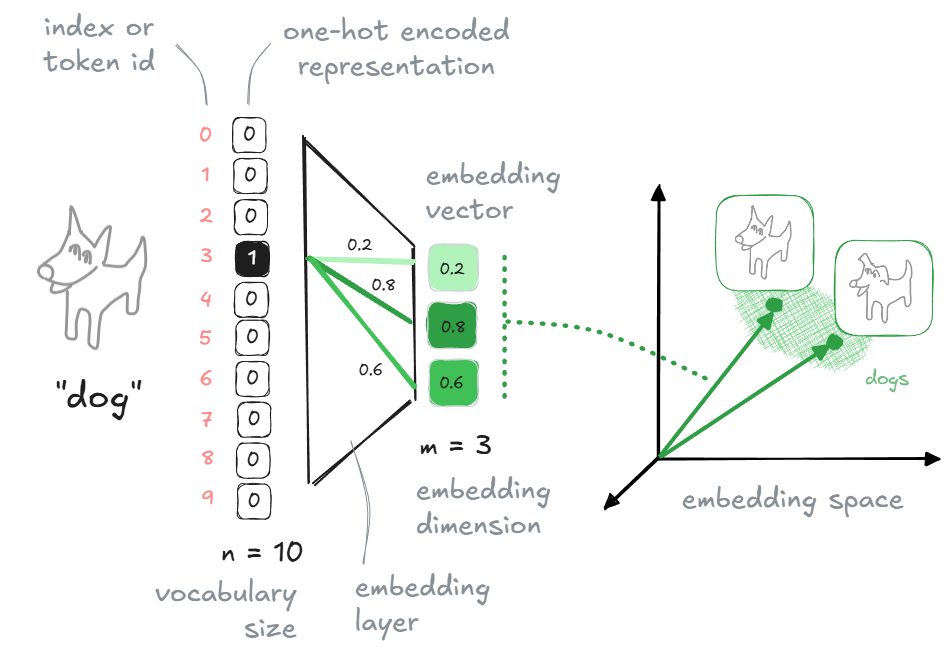 A word/token can be represented as a one-hot vector (sparse) or as an embedding vector (dense). Embedding vectors allow to capture semantics in their directions and make possible a more efficient processing. Image by the author.
By the way, embeddings can be created for images, too, as I explain in this post on diffusion models. In general, they have some very nice properties:
- They build up a compact space, in contrast to the sparse one-hot vector space.
- They are continuous and differentiable.
- If semantics are properly captured, words with similar meanings will point in similar directions. As a consequence, we can perform arithmetic operations with them, such that algebraic operations (
+, -) can be applied to words; for instance, the wordqueenis expected to be close toking - man + woman.
 Embeddings can be computed for every modality (image, text, audio, video, etc.); we can even create multi-modal embedding spaces. If the embedding vectors capture meaning properly, similar concepts will have vectors to similar directions. As a consequence, we will be able to apply some algebraic operations on them. Image by the author.
── ◆ ──
The original Transformer was designed for language translation and it has two parts:
- The encoder, which converts the input sequence (e.g., a sentence in English) into hidden states or context.
- The decoder, which generates an output sequence (e.g., the translated sentence in Spanish) using as guidance some of the output hidden states of the encoder.
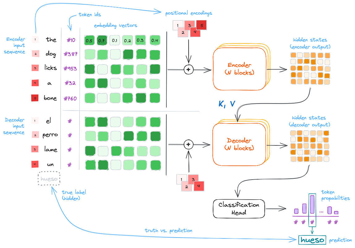 Simplified architecture of the original Transformer designed for language translation. Highlighted: inputs (sentence in English), outputs (hidden states and translated sentence in Spanish), and main parts (the encoder and the decoder).
Using as reference the figure above, here’s how the Transformer works:
-
The encoder and the decoder are subdivided in
Nencoder/decoder blocks each; these blocks pass their hidden state outputs as inputs for the successive ones. -
The input of the first encoder block are the embedding vectors of the input text sequence. Positional encodings are added in the beginning to inject information about token order, since the self-attention layers inside the blocks (see next section) are position-agnostic. In the original paper, positional encoding vectors were $\mathbf{R} \rightarrow \mathbf{R}^n$ sinusoidal mappings: each unique scalar yielded a unique and different vector, thanks to systematically applying sinusoidal functions to the scalar. However, in practice learned positional embeddings are often used instead.
-
For the translation task the encoder input contains the representation of the full original text sequence; meanwhile, the decoder produces the output sequence token by token, but it always has access to the full and final encoder hidden states (the context).
-
The decoder blocks work in a similar way as the encoder blocks; the last decoder block produces the final set of hidden states, which are mapped to output token probabilities using a linear layer followed by a softmax function (i.e., we have a classification head over the vocabulary).
Soon after the publication of the original encoder-decoder Transformer designed for the language translation task, two related, important Transformers were introduced:
- BERT: Pre-training of Deep Bidirectional Transformers for Language Understanding (Devlin et al., 2018), which is an implementation of the encoder-only part of the original Transformer.
- GPT: Improving Language Understanding by Generative Pre-Training (Radford et al., 2018), an implementation of the decode-only part of the original Transformer.
BERT-like encoder-only transformers are commonly used to generate feature vectors $x$ of texts which can be used in downstream applications such as text or token/word classification. If the Encoder is trained separately, the sequence text is shown to the architecture with a masked token which needs to be predicted. This scheme is called masked language modeling.
GPT-like decoder-only transformers are commonly used as generative models to predict the next token in a sequence, given all the previous tokens (i.e., the context, which includes the prompt). During training, the model is shown sequences of text and learns to predict each token based on the preceding ones.
The full encoder-decoder architecture is not as common as the other two currently, but it is used in some specific models for text-to-text tasks, such as summarization and translation. Examples include T5 (Raffel et al., 2019) and BART (Lewis et al., 2019).
Deep Dive into the Transformer Architecture
So far, we’ve seen the big picture of the Transformer architecture and its subtypes (encoder-decoder, encoder-only, decoder-only).
But what’s inside those encoder and decoder blocks? Just Attention, normalization, and linear mappings. Let’s see them in detail.
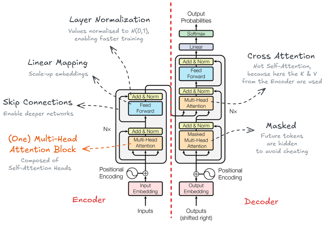 The Transformer architecture with all its components. Image from the orinal paper by Vaswani et al. (2017), modified by the author.
As we can see in the figure above, each of the N encoder and decoder blocks are composed of the following sub-components:
-
Multi-Head Self-Attention modules: The core component of the Transformer. It allows the model to focus on different parts of the input sequence when processing each token. Multiple attention heads enable the model to capture various relationships and dependencies in the data. More on this below

- Skip connections, Add & Norm: These are residual (skip) connections followed by layer normalization. Residual connections help to avoid vanishing gradients in deep networks by allowing gradients to flow directly through the skip connections. Normalizing the inputs across the features dimension stabilizes and accelerates training.
- Feed-Forward Neural Network (FFNN, i.e., several concatenated linear mappings): A fully connected feed-forward network applied independently to each position. It consists of two linear transformations with a ReLU activation in between, allowing the model to learn complex representations.
The key contribution of the Transformer architecture is the Self-Attention mechanism. Attention was introduced by Bahdanau et al. (2014) and it allows the model to weigh the importance of different tokens in the input sequence when processing each token. In practice for the Transformer, similarities of the tokens in the sequence are computed simultaneously (i.e., dot product) and used to weight and sum the embeddings in successive steps.
We can see there are different types of attention modules in the Transformer:
- Self-Attention in the encoder blocks: Each token attends to the similarities of all tokens in the input sequence. It’s called self-attention, because the similarities of the input tokens only are used, i.e., without any interaction with the decoder. For more information, keep reading below.
- Masked Self-Attention in the decoder blocks: Each token attends to all previous tokens in the output sequence (masked to prevent attending to future tokens).
- Encoder-Decoder Cross-Attention in the decoder blocks: Each token in the output sequence attends to all tokens in the encoder-input sequence. In other words, all final hidden states from the encoder are used in the attention computation.
Additionally, each attention module is implemented as a Multi-Head Attention mechanism. This means that multiple attention heads are used in parallel. The following figure shows brief overview of how this works.
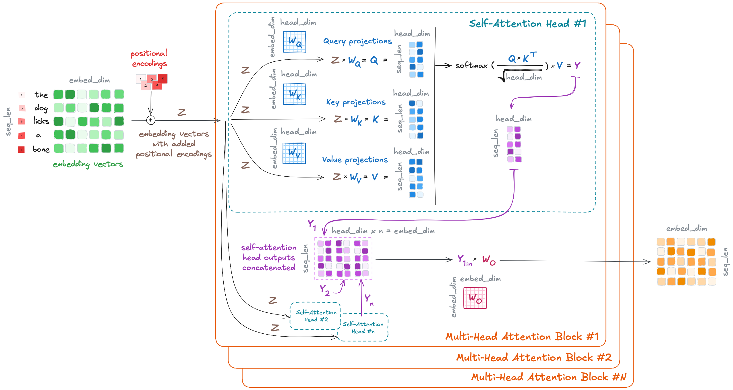 The LLM (Self-)Attention module, annotated. Image by the author.
The Self-Attention Head is the core implementation of the attention mechanism in the Transformer. Each multi-head attention module contains $n$ self-attention heads, which operate in parallel. The input embedding sequence $Z$ is passed to each of these $n$ self-attention heads, where the following occurs:
- We transform the original embeddings $Z$ into $Q$ (query), $K$ (key), and $V$ (value). The transformation is performed by linear/dense layers ($W_Q$, $W_K$, $W_V$), which consist of the learned weights. These query, key, and value variables come from classical information retrieval; as described in NLP with Transformers (Tunstall et al., 2022), using the analogy to a recipe they can be interpreted as follows:
- $Q$, queries: ingredients in the recipe.
- $K$, keys: the shelf-labels in the supermarket.
- $V$, values: the items in the shelf.
- $Q$ and $K$ are used to compute similarity scores between token embeddings (self dot-product), and then we use those similarity scores to weight the values $V$, so the relevant information is amplified. This can be expressed mathematically with the popular and simple attention formula:
\(Y = \mathrm{softmax}(\frac{QK^T}{\sqrt{d_k}})V,\)
where
- $Y$ are the contextualized embeddings,
- and $d_k$ is the dimension of the key vectors (used for scaling), which is the same as the embedding size divided by the number of heads (head dimension).
Then, these $Y_1, …, Y_n$ contextualized embeddings are concatenated and linearly transformed to yield the final output of the multi-head attention module. The output of the first multi-head self-attention module is the input of the next one, and so on, until all $N$ blocks process embedding sequences. Note that the output embeddings from each encoder block have the same size as the input embeddings, so the encoder block stack has the function of transforming those embeddings with the attention mechanism.
I hope it is now clear why the Transformer paper is titled Attention Is All You Need: It turns out that successively focusing and transforming the embeddings via the attention mechanism produces the magic in the LLMs.
Finally, let’s see some typical size values, for reference:
- Embedding size: 768, 1024, …, 2048.
- Sequence length (context, number of tokens): 128, 256, …, 8192.
- Number of layers/blocks, $N$: 12, 24, 36, 48.
- Number of attention heads, $n$: 12, 16, 20, 32.
- Head dimension: typically, embedding size divided by number of heads.
- Feed-Forward Network (FFN) inner dimension: 2048, 4096, …, 10240.
- Vocabulary size, $m$: 30,000; 50,000; 100,000; 200,000.
- Total number of parameters: from 110 million (e.g., BERT-base) to 175 billion (e.g., GPT-3), and much more!
Using the Transformer Outputs
There are many ways in which the outputs of the Transformer can be used, depending on the task and the architecture (some of these ways were mentioned above already):
- Encoder-decoder models (e.g., T5 (Raffel et al., 2019)) have been used for text-to-text tasks, such as translation and summarization. However, big enough decoder-only models (e.g., GPT-3 (Brown et al., 2020)) have shown remarkable performance in these tasks, too, and have become more popular nowadays.
- Encoder-only models (e.g., BERT (Devlin et al., 2018)) are commonly used to generate feature vectors of texts, which can be used in downstream applications such as text or token/word classification, or even regression. We just need to attach the proper mapping head to the output of the encoder (e.g., a linear layer for classification) and fine-tune the model on the specific task.
- Decoder-only models (e.g., GPT-3 (Brown et al., 2020)) are commonly used as generative models to predict the next token in a sequence, given all the previous tokens (i.e., the context, which includes the prompt).
Probably, the most common way to interact with LLMs for the layman user is the latter: decoder-only generative models. As mentioned, these models generate one word/token at a time, so we feed their outputs back as inputs for successive generations (hence, they are called autoregressive). In that scheme, we need to consider the following questions:
- Which tokens are considered as candidates every generation? (token sampling)
- What strategy is used to select and chain the tokens? (token search during decoding)
Recall that the output of the generative model is an array of probabilities, specifically, a float value $p \in [0,1]$ for each item in the vocabulary set $V$. A naive approach would be to
- consider all token probabilities as candidates ${p_1, p_2, …}$ (full distribution sampling),
- and select the token with the highest probability at each generation step: $\mathrm{token} = V(\mathrm{argmax}{p_1, p_2, …})$ (greedy search decoding).
However, such a naive approach often leads to repetitive and dull text generation, as described by Holtzman et al. (2019). To mitigate this issue, these parameters and strategies are often used:
- Temperature: we apply the softmax function to the output logits $z_i = \mathrm{ln}(p_i)$ by using a temperature variable $T$ in the exponent (Boltzman distribution): $p_i’ = \mathrm{softmax}(z_i / T)$. That changes the $p$ values as follows:
- $T = 1$: no change, same as in the original output.
- $T < 1$: small $p$-s become smaller, larger $p$-s become larger; that means we get a more peaked distribution, i.e., less creativity and more coherence, because the most likely words are going to be chosen.
- $T > 1$: small $p$-s become bigger, larger $p$-s become smaller; that yields a more homogeneous distribution, which leads to more creativity and diversity, because any word/token could be chosen.
- Top-$k$ and top-$p$: instead of considering all tokens each with their $p$ (with or without $T$), we reduce it to the $k$ most likely ones and select from them using the distribution we have; similarly, with a top-$p$, we can select the first tokens that cumulate up to a certain $p$-threshold and choose from them.
- Beam search decoding (as oposed to greedy search): we select a number of beams $b$ and keep track of the most probable next tokens building a tree of options. The most likely paths/beams are chosen, ranking the beams with their summed log probabilities. The higher the number of beams, the better the quality, but the computational effort explodes. Beam search sometimes suffers from repetitive generation; one way to avoid that is using n-gram penalty, i.e., we penalize the repetition of n-grams. This is commonly used in summarization and machine translation.
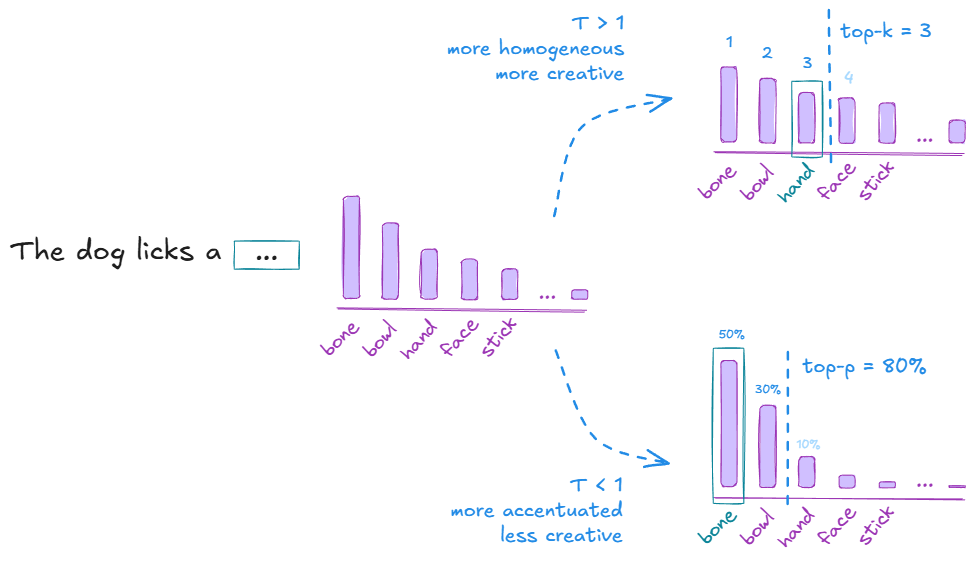 Token sampling strategies in LLMs. The LLM outputs a probability for each of the tokens in the vocabulary. If we apply a temperature T, top-k, or top-p strategy, we modify the distribution from which the next token is sampled. With T > 1, the distribution becomes more uniform, leading to more diverse outputs (since tokens have a more similar probability); in contrast, with T < 1, the distribution becomes more peaked, leading to more focused and coherent outputs. If we set top-k to be 3, we only consider the three most likely tokens for sampling; similarly, with a top-p threshold of 80%, we consider the smallest set of tokens whose cumulative probability is at least 80%. Image by the author.
Additional Relevant Concepts
My goal with this post was to explain in plain but still technical words how LLMs work internally. In that sense, I guess I have already given the best I could and I should finish the text. However, there are some additional details that probably fit nicely as appendices here. Thus, I have decided to include them with a brief description and some references, for the readers who optionally want to go deeper into the topic.
── ◆ ──
Context Size — This refers to the maximum number of words/tokens that the model can consider as input at once, i.e., the input sequence length or seq_len. If we look at the attention mechanism figure above, we will see that the learned weight matrices are independent of the context size; however, the attention computation itself scales quadratically with sequence length due to the $QK^T$ operation. This is a major bottleneck in terms of memory and speed, and it’s the main reason why the initial LLMs had a fixed and shorter context size ($512$ - $4,096$ tokens). In recent years, the research community has explored new methods to alleviate that limitation, introducing techniques such as sparse attention, linearized attention, low-rank approximations, and other mathematical/architectural/system tricks. These enable larger context sizes (up to $1,000,000$ tokens in the case of Gemini Pro).
Distillation and Quantization — As their name indicates, Large Language Models are large, and that makes them difficult to deploy in production environments. Two techniques to overcome that are distillation and quantization. When we distill a model, we train a smaller student model to mimic the behavior of a larger, slower but better performing teacher (i.e., the original LLM). This is achieved, among other techniques, by using the teacher’s output probabilities as soft labels when training the student. A notable example of distillation is DistilBERT (Sanh et al., 2019), which achieves around 97% of BERT’s performance, but with 40% less memory and 60% faster inference. On the other hand, quantization consists in representing the weights with lower precision, i.e., float32 -> int8 ($32/8 = 4$ times smaller models). The models not only become smaller, but the operations can be done faster (even 100x faster), and the accuracy is sometimes similar.
Emergent Abilities — As described by Wei et al. (2022), “emergent abilities are those that are not present in smaller models, but appear in larger ones”. In other words, they are capabilities that arise, but which were not explicitly trained. This often referred to as zero-shot or few-shot learning, because the model can perform tasks without any or with very few examples, as demonstrated by GPT-3 (Brown et al., 2020), and they start to appear in the 10-100 billion parameter range (GPT-3 had 175 billion parameters). Examples of emergent abilities include arithmetic, commonsense reasoning, and even some forms of creativity.
Scaling Laws — Kaplan et al. published in 2020 the interesting paper Scaling Laws for Neural Language Models, which describes how the performance of language models scales. They discovered that there is a power-law relationship between the model’s performance measured in terms of loss $L$, the required compute $C$, the dataset size $D$ and the model size $N$ (number of parameters): $L(X) \sim X^{-\alpha}$, with $X \in {N, C, D}$ and $\alpha \in [0.05, 0.1]$. In other words, when model size $N$, dataset size $D$, or training compute $C$ are scaled independently (and are not bottlenecks), the training loss $L$ decreases approximately as a power law of each quantity. In that sense, we can use these scaling laws to extrapolate model performance without building them, but theoretically! Similarly, for a fixed compute budget, there is an optimal trade-off between model size and dataset size. These insights led to the development of more efficient training strategies and architectures, such as the ones explored in the Chinchilla study (Hoffman et al., 2022), which suggest that smaller models trained on more data can achieve better performance than larger models trained on less data. Finally, note that training compute is roughly proportional to $6 \times N \times D$, while inference compute scales linearly with model size and generated sequence length.
RLHF: Reinforcement Learning with Human Feedback — OpenAI presented InstructGPT (Ouyang et al., 2022) shortly before releasing their popular ChatGPT. This paper explains how the initial chatbot model GPT 3.5 was aligned with human preferences using reinforcement learning. They followed 3 major steps: (1) First, a GPT model was fine-tuned with human-written conversation input-output pairs. (2) Then, the GPT model produced several answers to a set of prompts and human annotators ranked these outputs from best to worst. These annotations were used to train a reward model (RM) to automatically predict the output score. (3) Finally, the GPT model (policy) was trained using the Proximal Policy Optimization (PPO) algorithm, based on the conversation history (state) and the outputs it produced (actions), and using the reward model (reward) as the evaluator.
PEFT: Parameter-Efficient Fine-Tuning — Low-Rank Adaptation of Large Language Models (or LoRA by Hu et al., 2021) consists in applying a mathematical trick during the fine-tuning of LLMs to make the process much more efficient. The pre-trained weight matrices $W$ are frozen and we add to them the new matrices $dW = A \cdot B$, which are the ones trained. These are factored as $dW = A \cdot B$, having $A$ and $B$ a much lower rank. The trick reduces trainable parameters by orders of magnitude and maintains or matches full fine-tuning performance on many benchmarks. Therefore, it has become a standard method for domain adaptation and instruction tuning. One popular implementation is the peft library from HuggingFace.
RAG: Retrieval Augmented Generation — LLMs have humongous amounts of general knowledge encoded in their parameters, but need to be fine-tuned for specific domains. That process is cumbersome and often inefficient, particularly when domain-specific information changes frequently. The work Retrieval-Augmented Generation (RAG) for Knowledge-Intensive NLP Tasks (Lewis et al., 2020) addressed such settings by using non-parametric information, i.e., they outsource the domain-specific memory. It works as follows: in an offline ingestion phase, the knowledge is chunked and indexed, often as embedding vectors. In the real-time generation phase, the user asks a question, which is encoded and used to retrieve the most similar indexed chunks; then, the LLM is prompted to answer the question by using the found similar chunks, i.e., the retrieved data is injected in the query. RAGs reduce hallucinations and have been extensively implemented recently.
Reasoning Models — Wei et al. showed that Chain-of-Thought Prompting Elicits Reasoning in Large Language Models (2022). In other words, prompting the model to think step by step improves its performance on math and reasoning tasks, suggesting that reasoning abilities are partly latent in large models. That simple yet powerful idea sparked research into prompting strategies and powered the fine-tuning with objectives that encourage multi-step inference, structured thinking, and tool use. One of the first popular open source reasoning models was DeepSeek-R1, but most of the current models have all improved reasoning capabilities, either by scale or via fine-tuning with reasoning objectives.
Agents — The improvement of reasoning capabilities and tool usage boosted the development of the so-called agentic workflows. An agent is basically an LLM which has tool access and is allowed to perform actions, e.g., read our emails and do some processing with them, like classify or even answer the trivial ones. Libraries like LangChain and LangGraph have made it relatively easy to build multi-agent systems that perform increasingly complex workflows, and frameworks like OpenClaw have enabled the creation of personalized assistants. The future is being automated, and agents seem to be a key part of that — security issues aside.
Summary and Some Final Thoughts
Large Language Models are not magic. At their core, they are stacks of linear transformations, normalization layers, and attention mechanisms applied to sequences of embedding vectors. And yet, by scaling those simple components to unprecedented sizes (in terms of parameters, data, and compute) they exhibit capabilities that feel surprisingly powerful.
In this post, I have:
- Reviewed how text is converted into embedding vectors.
- Described the original encoder-decoder Transformer and its encoder-only and decoder-only variants.
- Taken a closer look at the self-attention mechanism and multi-head attention.
- Discussed how decoding strategies such as temperature, top-$k$, top-$p$, and beam search influence text generation.
- Briefly touched on important side concepts such as context length, scaling laws, RLHF, PEFT/LoRA, RAG, reasoning models, and agents.
If you want to go deeper into the topic, I recommend the following resources:
- The original paper: Attention Is All You Need (Vaswani et al., 2017)
- My notes of the great book NLP with Transformers (Tunstall et al., 2022)
- The Illustrated Transformer (Jay Alammar)
- The Annotated Transformer (Harvard NLP)
- A minimal PyTorch re-implementation of the OpenAI GPT (Andrej Karpathy)
── ◆ ──
LLMs have increased my productivity significantly. I use them extensively for research, text editing, and programming. However, I still think that they are expert systems for experts: when used without proper guidance, the quality of their output can be quite mediocre — and in some cases, even worse: I have seen many instances of dull AI-generated texts and bloated, unmaintainable code. I am aware, of course, that they are improving at a rapid pace, though.
Overall, I am optimistic. In the same way that the Internet increased our overall productivity — while replacing some jobs and creating new ones — I think LLMs will probably have a similar (or even greater) net-positive effect. For instance, I do not believe that Software Engineers will disappear. Rather, they will likely shift toward tasks related to architecture, orchestration, integration, and maintenance. Junior roles and inexperienced professionals seem to be the most affected at the moment, but they will also be able to learn faster with these tools than we did before. As the ecosystem stabilizes, they may end up being in even higher demand. And, at the end of the day, everyone will want a human responsible for any AI-generated outcome.
I am confident that we will find ways to mitigate risks such as dependence, personal data harvesting and automated control/surveillance, just as we invented gyms to stay fit and healthy, or engineered locks and cryptographic systems to protect our privacy. At the moment, it is hard for me to believe that a Transformer-based model can intentionally go rogue and cause harm on its own, because I cannot conceive of any consciousness in them — at least not in the sense of “I am aware that I exist here and now, and I have some purpose and agency”. I see LLMs as systems that simulate patterns from their training data. In contrast, humans maintain (and constantly update) a world model, and use language as a tool to interact with that world model. An LLM has no internal state and it can’t learn in real-time — it can only simulate “small breaths” by producing tokens; one could even argue that it even “dies” after producing each token, or at least once the final <STOP> token is emitted.
At the same time, granting an LLM-based agent unrestricted access to personal information and powerful tools could indeed be irresponsible — perhaps comparable to giving a monkey a machine gun. Yet we have faced similar situations in the past: when technologies become powerful, we introduce safeguards, norms, and regulation to govern their use.
Let’s see what the future awaits us. I believe it will be exciting, and that we will find ways to navigate the limitations and risks of this technology, as we’ve done in the past.
How have LLMs impacted your life? How do you think they will change the world in the next 5-10 years?